Conditional Independence, d-Separation, Markov Property and Markov Blanket
This post is largely inspired by the following lectures:
Also, the topics I mention here are pretty abstract and I do not provide any examples to make it more intuitive. I encourage interested readers to follow the lecture series from UC Berkeley (by Prof. Dan Klein) for some nice examples.
Conditional Independence
Before going into this topic, it is better to review the concept of independence between random variables. Suppose $a$ and $b$ are two random variables and they respectively follow the probability distribution $p(a)$ and $p(b)$. We can say $a$ and $b$ are independent if,
\[p(a,b)=p(a) p(b)\]where, $p(a,b)$ is the joint distribution of $a$ and $b$.
This can be generalized to more than two random variables.
To formulate the framework for conditional independence, we need three random variables $a$, $b$, and $c$. Suppose they follow the probability distribution $p(a)$, $p(b)$ and $p(c)$. We say random variables $a$ and $b$ are conditionally independent given $c$ if the following expression is true in general:
\[p(a,b|c) = p(a|c) p(b|c)\]Conditional Independence in Directed Graphical Model
First of all, let’s summarise the concept of a directed graphical model. In short, it presents the dependencies among random variables through a directed acyclic graph, where nodes correspond to variables and directed edges indicate direct influences between them. Now to understand the conditional independence in the context of PGM, we need to consider the three elemental structures.
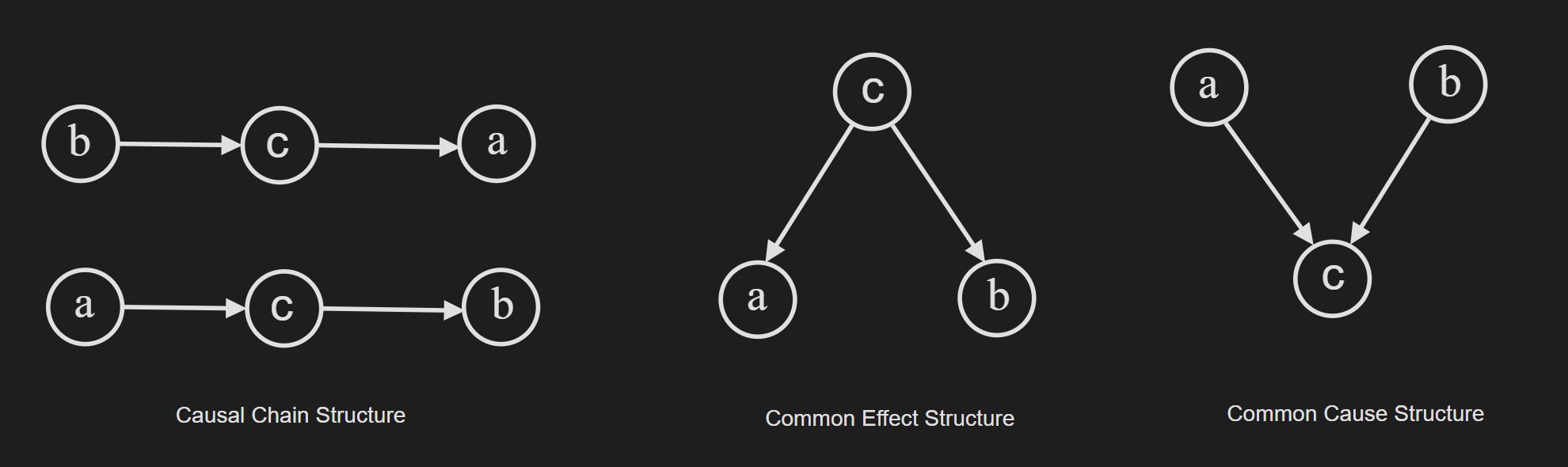
The names for these three elemental structures are “Causal Chain Structure”, “Common Effect Structure” and “Common Cause Structure”. In a large probabilistic graphical model (PGM), you can break down the PGM into these “triplet” structures and make deductions about the dependence of random variables.
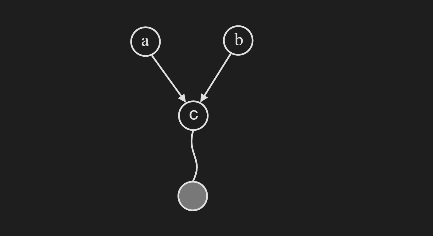
Common Effect Structure
First let’s try to understand the reasoning behind the name. According to the diagram below, the random variable $c$ is influncing both the random variable $a$ and $b$. 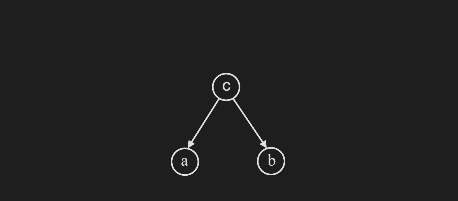
Now if we consider the case when $c$ is not observed, we can break down the joint probability distribution as follows:
\[p(a,b,c)=p(c)p(a|c)p(b|c)\]If we write down $p(a,b)$ by trying to integrate out $c$, we can easily see that $p(a,b)$ can not be factored in $p(a)$ and $p(b)$.
\[p(a, b)=\sum_c p(a, b, c)=\sum_c p(c) p(a \mid c) p(b \mid c) \neq p(a) p(b)\]
Now if we consider the case when $c$ is observed, we can prove with Bayes theorem that $a$ and $b$ are conditionally independent given $c$.
\[p(a, b \mid c)=\frac{p(a, b, c)}{p(c)} = \frac{p(c) p(a \mid c) p(b \mid c)}{p(c)} =p(a|c) p(b \mid c)\]Intuitively this means, if we are able to completely observe $c$, the random variable $a$ and $b$ are no longer dependent.
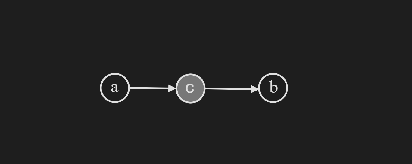
Causal Chain Structure
The naming is pretty easy to understand based on the following diagram. It is a chain of random variables where one random variable is dependent on the random variable before it. Another way to phrase this is one random variable is causing a influence to another random variable.
Now we can break down the joint distribution as follows:
\[p(a,b,c) = p(a) p(c|a) p(b|c)\]If we proceed by applying Bayes theorem,
\[p(b|a,c)= \frac{p(a,b,c)}{p(a,c)} = \frac{ p(a) p(c|a) p(b|c)}{p(a)p(c|a)}= p(b|c)\]This means conditioning on $a$ does not have any effect on $b$. In other words, $a$ and $b$ are conditionally independent given $c$.
This is sometimes referred to as “Evidence along a chain breaks the chain”. Another way to think about it is, that conditioning on something in the middle, blocks the flow of dependency between random variables.
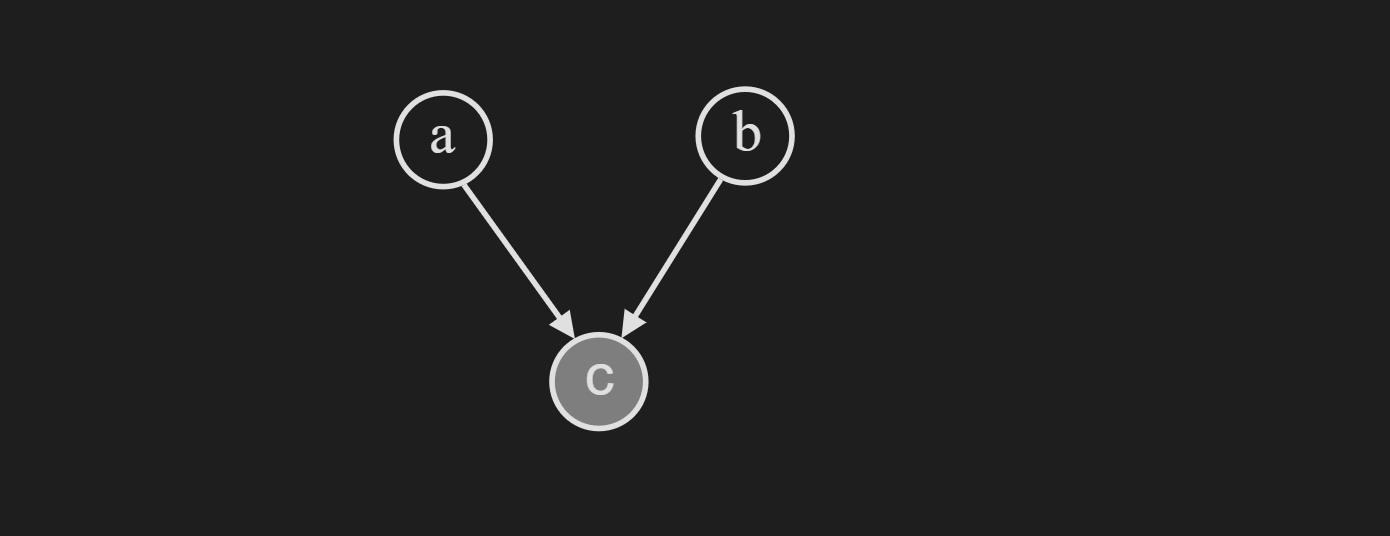
Common Cause Structure
Note that, this is sometimes referred to as “collider” structure.

We can break down the joint probability distribution expression as follows:
\[p(a,b,c) = p(a) p(b) p(c|a,b)\]Now we try to find $p(a,b)$ by trying to integrate out $c$ we get the following:
\[p(a,b) = \sum_{c} p(a) p(b) p(c|a,b)= p(a) p(b) \sum_{c} p(c|a,b) = p(a) p(b)\]This means $p(a,b)$ are independent in this common cause structure. Let’s see what happens when we condition on $c$.
We fail to make the $a$ and $b$ conditionally independent after conditioning on $c$.
This holds when we condition on any descendent of $c$.
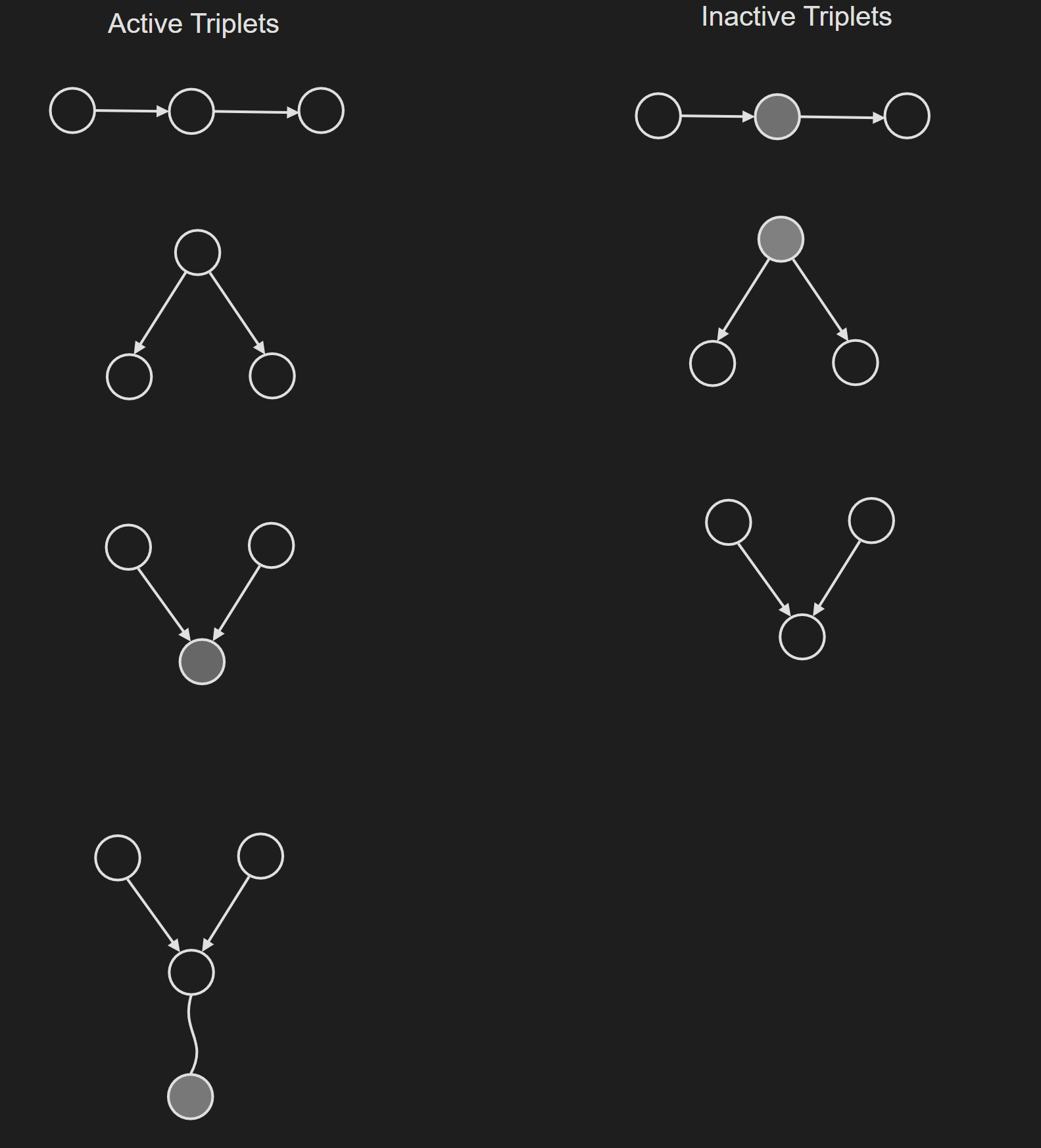
To summarise, these examples introduce the notion of active trails and blocked trails in directed graphical models.
d-Separation
The d-Separation formalizes the above concepts into a nicely structured algorithm. The algorithm answer the question to query which is given below:
\[\text { Query: } x_i \perp x_j \mid\left\{x_{k_1}, \ldots, x_{k_n}\right\}\]To answer the query we need to follow the steps mentioned below:
\[\text { Check all paths between } x_i \text { and } x_j\]If one or more paths are active, then independence is not guaranteed \(x_i \not \perp x_j \mid\left\{x_{k_1}, \ldots, x_{k_n}\right\}\)
Otherwise (i.e. if all paths are inactive), then “D-separated” = independence is guaranteed \(x_i \perp x_j \mid\left\{x_{k_1}, \ldots, x_{k_n}\right\}\)
Markov Blanket in Directed Graphical Model
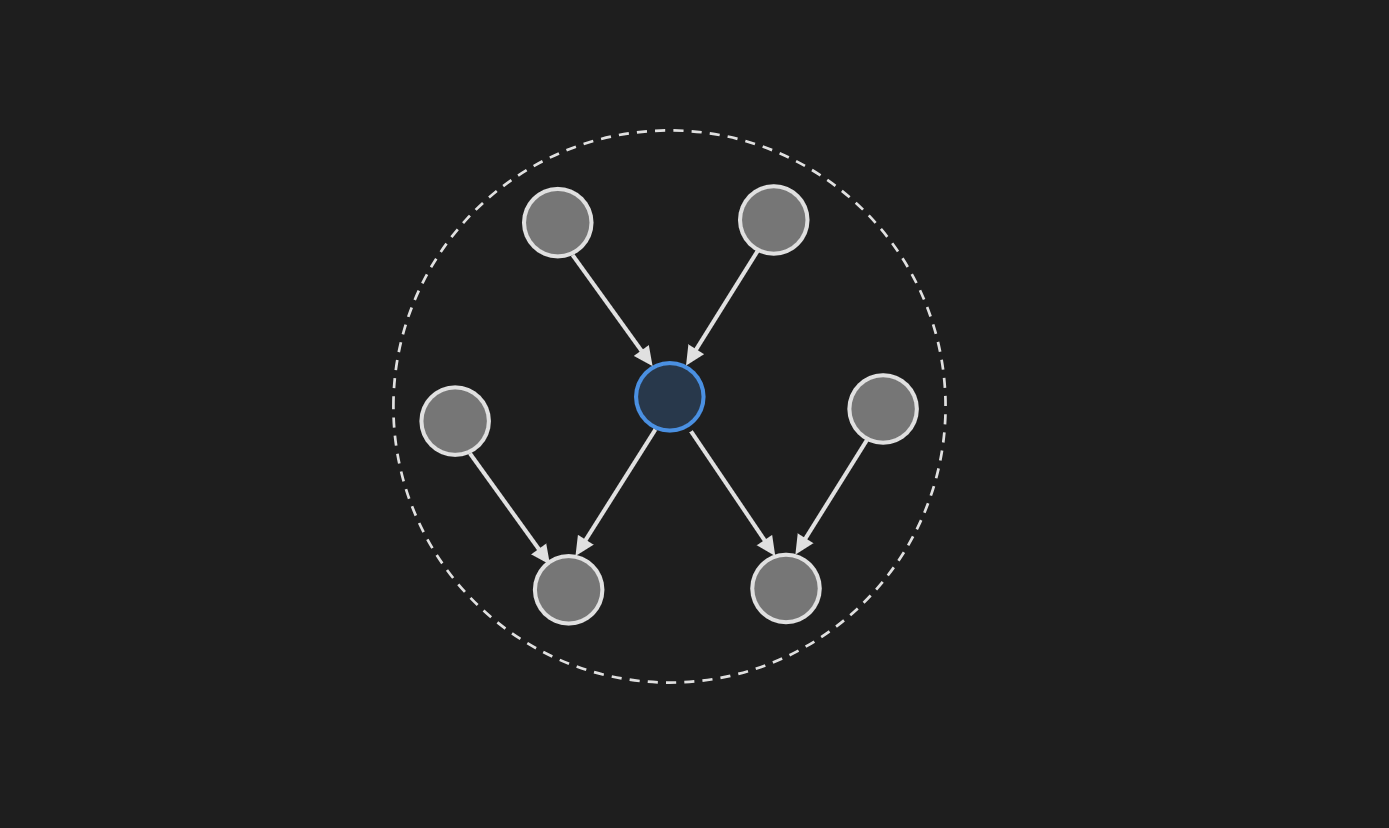
A node’s Markov blanket includes all its parents, children, and children’s parents. Given that we observed its parents, children, and children’s parents, the node becomes independent from all the other nodes in the graph. Mathematically, that can be expressed as:
\[P(x \mid \mathcal{X} \backslash\{x\})=P(x \mid MB (x))\]where, $MB(x)$ is the Markov blanket consisting of the node’s parents, children, and children’s parents and $\mathcal{X}$ is the node set excluding $x$. Mathematically, $MB(x)$ can be more explicitly written as:
\[MB(x)=Parents(x) \cup Children(x) \cup Parents (\text Children (x))\]Markov Random Field
Undirected graphical models are also known as Markov random fields. To understand them, you need to understand concepts like potential functions, cliques, maximal cliques, partition functions, etc. But I am not going to go over them in this article.
Local Markov Property in Markov Random Field
When conditioned on its neighbors, $x$ becomes independent of the remaining variables of the graph. Mathematically, it can be written as,
\[p(x \mid \mathcal{X} \backslash\{x\})=p(x \mid n e(x))\]Where, $\mathcal{X}$ is the node set excluding $x$ and $ne(x)$ is the neighbor node set of $x$. In other words, when we know about the neighboring nodes of $x$, knowing about the rest of the nodes does not provide any additional information. Let’s make it concrete with a visual example,
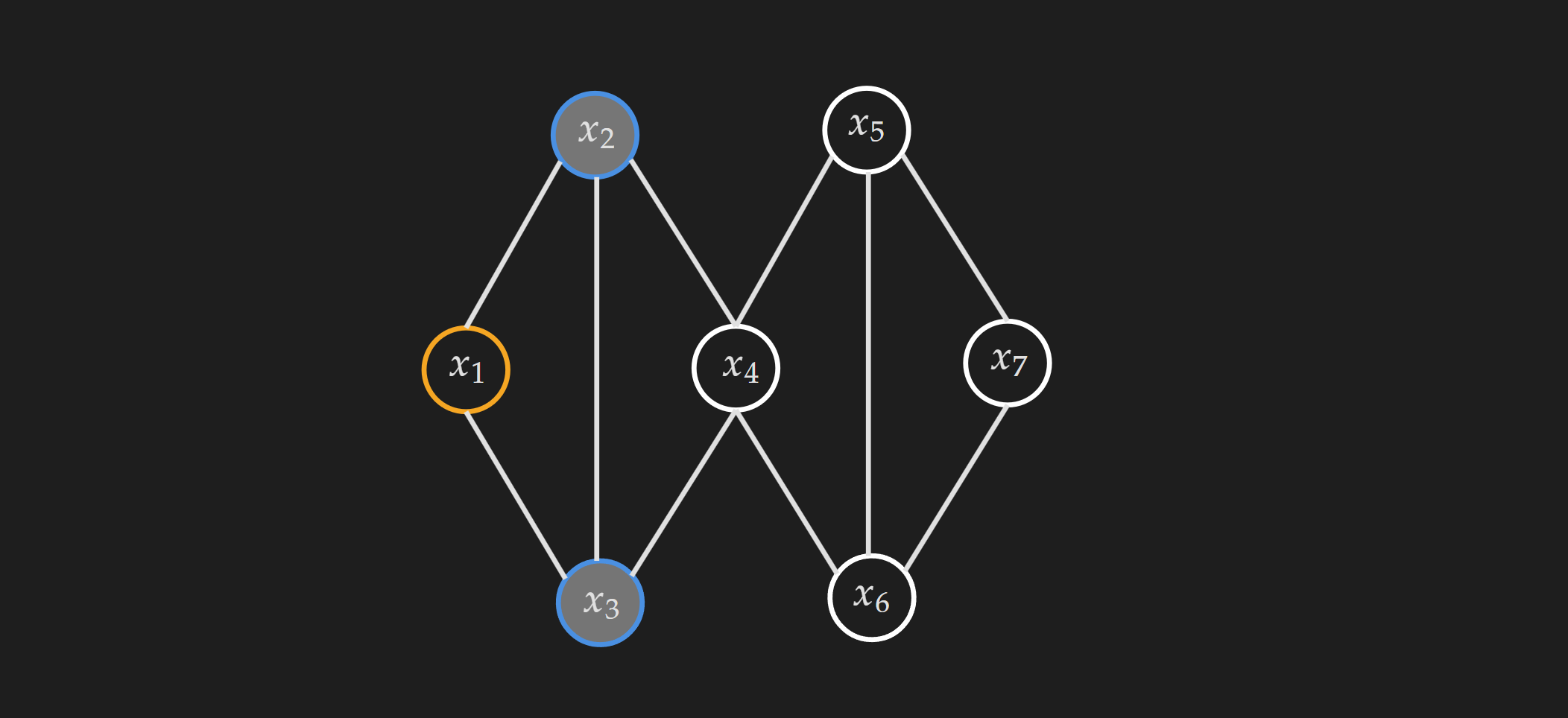
Suppose, in the above MRF we condition on the neighbors of $x_1$, where $ne(x_1)={ x_2, x_3}$. In that case, $x_1$ is independent of all the other nodes in the graph which are $x_4, x_5,x_6, x_7$.
Pairwise Markov Property in Markov Random Field
For an MRF, if $x_i$ and $x_j$ are not directly connected by an edge, given the values of all other nodes in the graph, $x_i$ and $x_j$ are conditionally independent. Mathematically that can be expressed as the following:
\[x_i \perp x_j~| \mathcal{X}\backslash \{x_i,x_j \}\]This is just a way to infer conditional independence between two nodes in an MRF.
Global Markov Property in Markov Random Field
The following MRF will be used to illustrate the global Markov property.
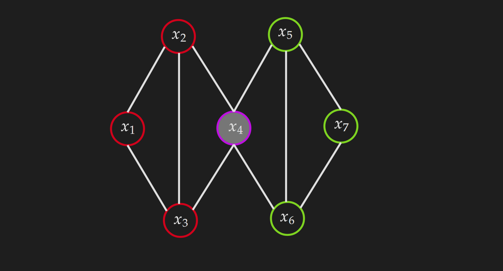 For disjoint sets of variables $(\mathcal{A}, \mathcal{B}, \mathcal{S})$ where $\mathcal{S}$ separates $\mathcal{A}$ from $\mathcal{B}$, we have $\mathcal{A} \perp \mathcal{B} \mid \mathcal{S}$. Let’s make it concrete with a visual example.
\(\mathcal{S}=\left\{x_4\right\}\) \(\mathcal{A}=\left\{x_1, x_2, x_3\right\}\) \(\mathcal{B}=\left\{x_5, x_6, x_7\right\}\)
If we condition on $x_4$, then all the nodes from $\mathcal{A}$ become independent from all the nodes in $\mathcal{B}$.
Markov Blanket in Markov Random Field
The notion of a Markov blanket in MRF can be derived from the local Markov property. The Markov blanket of a node $x$ is the neighbor node set of the node $x$ i.e. $ne(x)$. Mathematically,
\[p(x \mid \mathcal{X} \backslash\{x\})=p(x \mid n e(x))\]