Kullback–Leibler Divergence

There are two ways to introduce KL divergence, one is with the notion of “distance between distributions” and another is with information theory. The latter one is more in line with what is really captured by KL divergence; but requires a lot of fundamental prerequisite concepts like entropy, mutual information, etc. Hence, I will introduce it with the first approach and then connect it back to the information-theoretic approach.

“Distance” between two distributions

Let consider a discrete random variable $X$ where the samples of the random variable are $X={x_{1},x_{2},x_{3},\cdots}$. Suppose there are two distribution $p_{\theta}$ and $q_{\phi}$. The subscript denotes the parameters of the distribution. One key thing to notice here, we are not claiming that the distribution is the same class of distributions because $\theta$ and $\phi$ are different. One can be a binomial distribution parameterized by $\theta$ and another can be poisson distribution parameterized by $\phi$.

For one specific sample of the distribution, we can compute the likelihood $p_{\theta}(x_{1})$ and $q_{\phi}(x_1)$. How do we measure the distance between these two evaluations? Think of them as two values in a number line. We can just take the difference between them to get a measure of “distance”. If the two distributions $p_{\theta}$ and $q_{\phi}$ are quite similar then the difference between $p_{\theta}(x_{1})$ and $q_{\phi}(x_1)$ should be low and vice versa.

But one important thing to keep in mind is, that we are dealing with a probability value, which is why it is better to take the $\log$ of these quantities first and then take the difference. This gives us $\log p_{\theta}(x_{1}) - \log q_{\phi}(x_{1})$ . But using the property of $\log$ we can get the following:-

\[\log \left( \frac{p_{\theta}(x_1)}{q_{\phi}(x_1)} \right)\]

which is called the log-likelihood ratio. Now, this is measuring “distance” for only sample $x_{1}$. We need to take into account all the samples $x_{1},x_{2},\cdots$ not just a single sample $x_{1}$. First, we can generalize the likelihood ratio by replacing index $1$ with $i$ and we get the following:

\[\log \left( \frac{p_{\theta}(x_i)}{q_{\phi}(x_i)} \right)\]

We can take the weighted average of this “distance measure” for all samples of the random variable $X$. You can think of it like we are averaging all individual log-likelihood ratio values for the random variable $X$. Following this logic, we can write :

\[\sum_{i=1} p_\theta\left(x_i\right) \log \left[\frac{p_\theta\left(x_i\right)}{q_\phi\left(x_i\right)}\right]\]

This is the definition of KL divergence. For continuous random variable we can replace $\sum$ with $\int$ to get the following:

\[\int_{i=1} p_\theta\left(x_i\right) \log \left[\frac{p_\theta\left(x_i\right)}{q_\phi\left(x_i\right)}\right]\]

For ease of writing it is conventional to drop $\theta$ and $\phi$ and just use $p$ and $q$ to refer to two separate distributions. Also, we don’t need to explicitly show the summation of over indices. This gives the following equation for discrete random variable:

\[\boxed{D_{KL}(p||q)= \sum_{x\in \mathcal{X}}p(x) \log \frac{p(x)}{q(x)}}\]

For continuous random variables the summation can be replaced by an integral sign and we get the following:

\[\boxed{D_{KL}(p||q)= \int_{x\in \mathcal{X}}p(x) \log \frac{p(x)}{q(x)}}\]

An example of KL divergence is shown in the diagram below. It is kind of self-explanatory if you know KL divergence is a measure of “distance” between distributions. When two distributions are not similar you should expect a larger value; whereas if the distributions are quite similar you should expect a lower value.

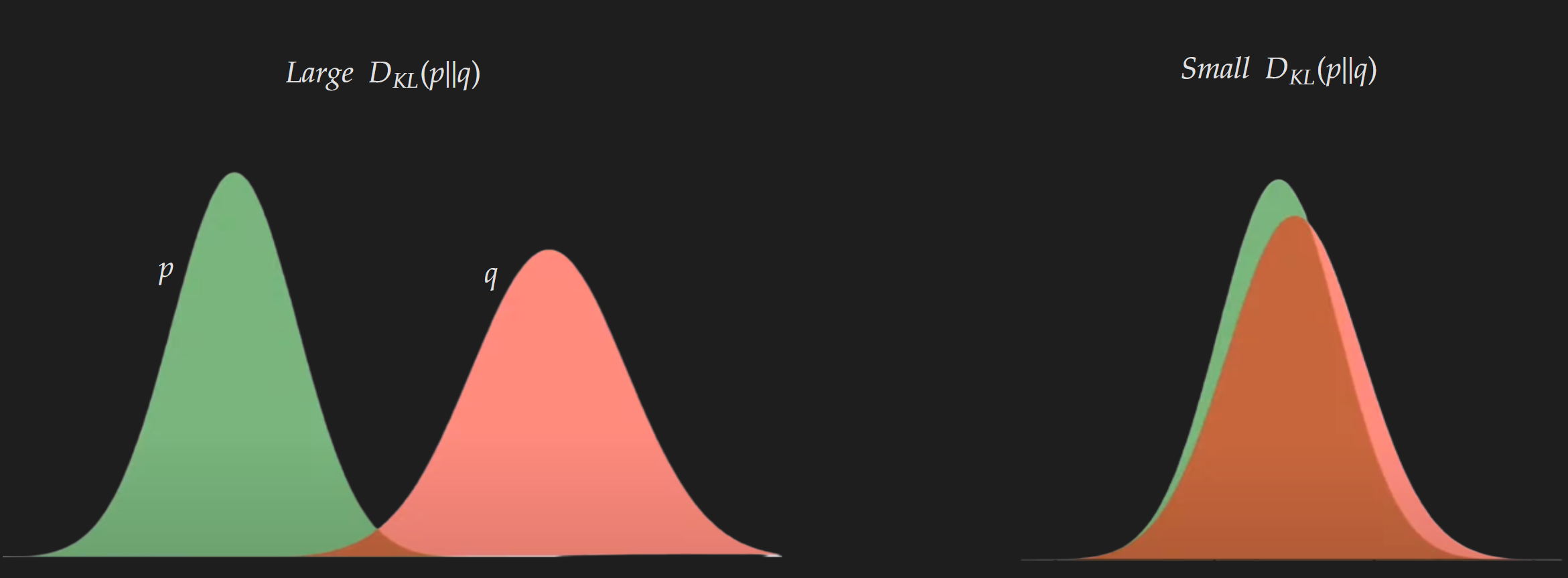
Even though the visualization is shown of one-dimensional distribution it is easily generalizable for higher dimensional distribution.

Why it is called “Divergence”?

One thing you might have noticed in the previous section I always used “ “ when using the word “distance”. It was intentional because KL divergence is not a true “distance” measure in the sense it is not symmetric. KL divergence between $p_{\theta}$ and $q_{\theta}$ will not be the same as the KL divergence between $q_{\theta}$ and $p_{\theta}$. In addition, it does not satisfy the triangle inequality. The unsymmetric nature can be mathematically expressed as below:

\[D_{KL}(p||q) \neq D_{KL}(q||p)\]

Also as it does not follow triangle inequality and hence we can write down the expression below:

\[D_{KL}(p \| q) \nleq D_{\mathrm{KL}}(p \| r)+D_{\mathrm{KL}}(r \| q)\]

KL Divergence is also a non-negative quantity i.e. $D_{KL}(p | q)\geq0$

Forward KL Divergence vs. Reverse KL Divergence

There are a couple of consequences due to the asymmetry property of KL divergence. To understand that, first, we need to understand the difference between “Forward KL Divergence” and “ Reverse KL divergence”. For this, we need to consider a practical setting like variational inference, where we have a target distribution (or true distribution) $p$ and we are trying to approximate a candidate distribution $q$. In this context, the forward KL divergence is given by :

\[D_{K L}(p \| q)=\mathbb{E}_{x \sim p}\left[\log \frac{p(x)}{q(x)}\right]\]

And the reverse KL divergence is given by:

\[D_{K L}(q \| p)=\mathbb{E}_{x \sim q}\left[\log \frac{q(x)}{p(x)}\right]\]

Let’s try to visualize what is happening by considering the distribution below as the true distribution $p$.

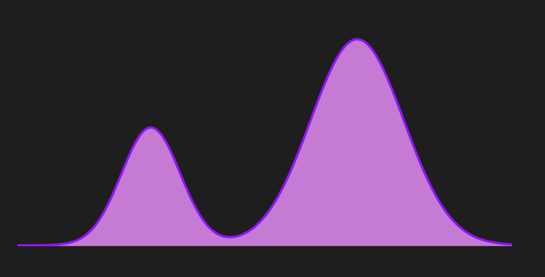
From the figure, we can see that $p$ is a bi-modal distribution. If we use forward KL divergence as a metric and use variational inference to approximate the parameterized distribution $q$ we will get something like below.

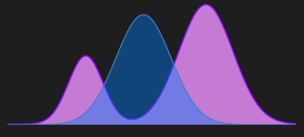
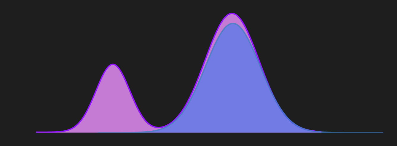
This shows that the forward KL exhibits mean-seeking behavior. In contrast, if reverse KL divergence is used as a metric it exhibits a mode-seeking behavior as shown in the following diagram.

Let’s look at an example of a 2D case:

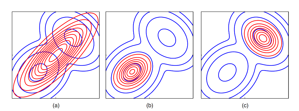Image taken from Bishop, C.M. and Nasrabadi, N.M., 2006. Pattern recognition and machine learning. The Left one is for Forward KL and the middle & the right one are for reverse KL.

Most people after learning this fact wonder which one is better or which one should be used; the forward KL divergence or the reverse KL divergence? The short answer is it depends. The first thing you need to come to terms with is, for higher dimensional distributions you can’t visualize what the hell is happening. Hence, there is no visual intuition to rely on and to decide which one you would want. In higher dimensions, the distribution might have $n$-number of modes and depending on the problem you are trying to solve, you might prefer the forward or the reverse KL divergence.

Connection to Information Theory

KL Divergence is also known as Relative Entropy and has a close connection to Mutual Information. Let’s start with the equation which connects mutual information to KL divergence:

\[\boxed{I(X; Y)=D_{K L}\left(p(x,y) \| p(x) p(y)\right)}\]

where $p(x) p(y)$ is the product between the marginal distribution between $p(x)$ and $p(y)$. The derivation of this specific equation is shown below:

\[\begin{aligned} I(X ; Y) & =H(Y)-H(Y \mid X) \\ & =-\sum_{y \in \mathcal{Y}} p(y) \log p(y)+\sum_{x \in \mathcal{X}, y \in \mathcal{Y}} p(x) p(y \mid x) \log p(y \mid x) \\ & =\sum_{x \in \mathcal{X}, y \in \mathcal{Y}} p(x, y) \log p(y \mid x)-\sum_{y \in \mathcal{Y}}\left(\sum_{x \in \mathcal{X}} p(x, y)\right) \log p(y) \\ & =\sum_{x \in \mathcal{X}, y \in \mathcal{Y}} p(x, y) \log p(y \mid x)-\sum_{x \in \mathcal{X}, y \in \mathcal{Y}} p(x, y) \log p(y) \\ & =\sum_{x \in \mathcal{X}, y \in \mathcal{Y}} p(x, y) \log \frac{p(y \mid x)}{p(y)} \\ & =\sum_{x \in \mathcal{X}, y \in \mathcal{Y}} p(x, y) \log \frac{p(y \mid x) p(x)}{p(y) p(x)} \\ & =\sum_{x \in \mathcal{X}, y \in \mathcal{Y}} p(x, y) \log \frac{p(x, y)}{p(y) p(x)} \\ & =D_{K L}(p(x,y) \| p(x) p(y)) \end{aligned}\]

This equation captures the “distance” between the joint distribution $p(x,y)$ and the product of marginal distributions $p(x)$ and $p(y)$. If the random variables $X$ and $Y$ are independent which means $p(x,y)=p(x) p(y)$, then $D_{K L}(p(x,y) | p(x) p(y)$ equals $0$ as per definition of KL divergence.

Connection to Cross-Entropy

To create the connection with cross-entropy first we need to start with the definition for KL divergence and perform some algebraic manipulations.

\[\begin{align*} D_{KL}(p||q) &= \sum_{x\in \mathcal{X}}p(x) \log \frac{p(x)}{q(x)} \\ &= \sum_{x\in \mathcal{X}}p(x)\log p(x) - p(x) \log q(x) \\ &= \sum_{x\in \mathcal{X}}p(x)\log p(x)- \sum_{x\in \mathcal{X}} p(x) \log q(x) \\ &=\underbrace{- \sum_{x\in \mathcal{X}} p(x) \log q(x)}_{\text{Cross-Entropy}}- \underbrace{\left(-\sum_{x\in \mathcal{X}}p(x)\log p(x) \right)}_{\text{Entropy}} \\ \end{align*}\]

This can be expressed as below where $H(p,q)$ is the cross-entropy between distribution $p$ and distribution $q$ \& $H(p)$ is the entropy of distribution $p$.

\[\boxed{D_{KL}(p||q) = H(p,q) - H(p)}\]

Let’s talk about how this formula is used in practice. First, swap the sides and define cross-entropy as below:

\[\underbrace{H(p,q)}_{\text{Cross-Entropy between $p$ and $q$}} = \underbrace{D_{KL}(p||q)}_{\text{KL Divergence between $p$ and $q$} }+ \underbrace{H(p)}_{\text{Entropy of distribution $p$}}\]

In the context of a supervised classification problem, it is a common practice to use cross-entropy as a cost function. You can think of $p$ as the true underlying data distribution and $q$ as the parameterized predicted distribution. The distribution $q$ is parameterized because it is controlled by the model parameters. One important thing to notice here, $H(p)$ equates to a constant value from an optimization perspective because it does not contain $q$.

References

[1] Ghosh, D. (2018). KL Divergence for Machine Learning. [online] The RL Probabilist. Available at: https://dibyaghosh.com/blog/probability/kldivergence.html.