Joint, Conditional and Marginal Entropy

Posted Aug 16, 2023 Updated Jul 5, 2024

By Dibaloke Chanda 6 min read

To understand the concept of mutual information first, we need to understand joint entropy, conditional entropy and marginal entropy. These concepts are not necessarily hard, but they are introduced poorly with just a bunch of equations thrown at the beginners.

Image taken from 3Blue1Brown video-Solving Wordle using information theory

Joint Entropy

Joint Entropy is nothing but the entropy of a joint distribution. The joint distribution can be constructed with multiple random variables. But to keep it simple, let’s consider a joint distribution of two random variables $X$ and $Y$. In addition, let’s keep the discussion limited to discrete random variables as that is easier to visualize and reason with. The joint entropy $H(X,Y)$ is given by the following equation:

\[\boxed{H(X, Y) = -\sum_{x \in \mathcal{X}} \sum_{y \in \mathcal{Y}} p(x, y) \log p(x, y)}\]

Sometimes the double summation is replaced by a single summation and written as follows:-

\[\boxed{H(X, Y) = -\sum_{x \in \mathcal{X}, \ y \in \mathcal{Y}} p(x, y) \log p(x, y)}\]

Now this equation essentially takes in a joint probability distribution $p(x,y)$ and spits out a single number that represents the expected information quantity in that joint distribution. Let’s start with a simple example, a joint distribution of a fair coin toss and a fair die roll. The assumption that needs to be made here the coin toss and die roll are independent of each other. The visualization of the distribution is shown below:

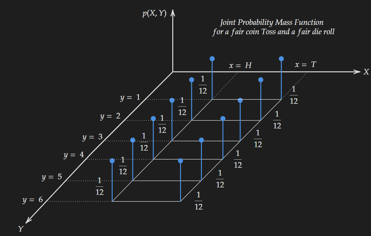
We can easily tell as the distribution is completely flat, which means it has a high joint entropy. We can compute it as follows (with $\log-e$ base) :

\[H(X,Y)= - 12 \times \frac{1}{12} \times \log(\frac{1}{12})=2.485\]

Now suppose we change the distribution by using a biased coin with a higher probability for “head” and the modified joint probability distribution is shown below:

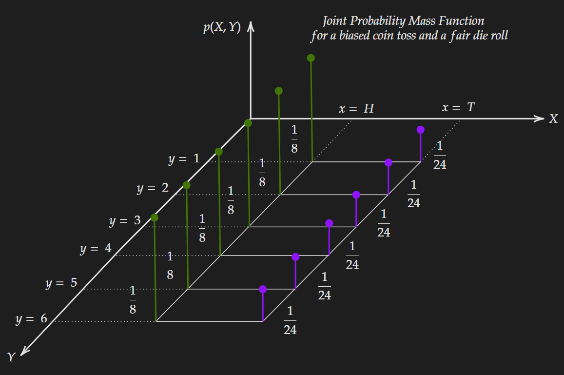
The computed entropy value for the modified joint distribution is given below:

\[H(X,Y)= - 6 \times \frac{1}{8} \times \log (\frac{1}{8}) - 6 \times \frac{1}{24} \times \log (\frac{1}{24})=2.354\]

As expected this is lower compared to the fair coin version.

We can generalize this concept for higher dimensional PMFs. The generalized version of the entropy formula for $n$ number of random variables $X_{1}, X_{2}, \cdots ,X_{n}$ is given below:

\[H(X_1, X_{2}, \cdots, X_n ) = -\sum_{x_1 \in \mathcal{X}_1, \ x_2 \in \mathcal{X}_2, \cdots, \ x_n \in \mathcal{X}_n} p(x_1, x_2,\cdots, x_n) \log p(x_1, x_2, \cdots, x_n)\]

which might look complex but essentially utilizes the same concept. It is no longer possible to visualize this with a diagram, but all the intuitions derived for two variables; hold for a multivariable case.

Conditional Entropy

Conditional entropy captures the expected information content in a conditional distribution. Let’s explain it with the same example given above.

Suppose we are given the fact that a coin toss results in “head”, which means we will be dealing with only a “slice” of the distribution i.e. a conditional distribution.

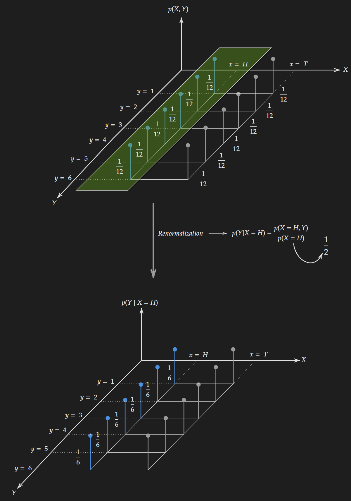Conditioning on random variable X (considering “Head” comes up)

We get the values after applying the following formula:

\[p(Y|X=H)= \frac{p(X=H,Y)}{p(X=H)}\]

Based on the conditional distribution we can compute the entropy as follows:

\[\begin{align*} H(Y|X=H) & = - \sum_{y \ \in \mathcal{Y}} p(Y=y|X=H) \log p(Y=y|X=H) \\ & = - 6 \times \frac{1}{6} \times \log \frac{1}{6} \\ & = 1.792 \end{align*}\]

The same thing can be done if $X=T$ and we compute the entropy as follows:

\[\begin{align*} H(Y|X=T) & = - \sum_{y \ \in \mathcal{Y}} p(Y=y|X=T) \log p(Y=y|X=T) \\ & = - 6 \times \frac{1}{6} \times \log \frac{1}{6} \\ & = 1.792 \end{align*}\]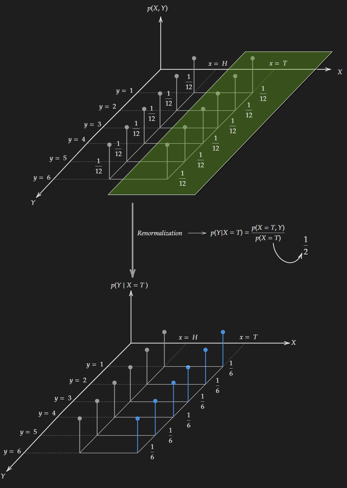

Conditioning on random variable X (considering “Tail” comes up)

But there is a slight issue, we are considering one case at a time, either “Head” or “Tail”.

We need to consider both the case of “Head” and “Tail” at once. One naive approach would be to add both $H(Y|X=H)$ and $H(Y|X=T)$ to get $H(Y|X)$. Though it seems reasonable, the issue with this approach is we are discarding the probability associated with a specific random variable. The right approach is to take the weighted average (expectation) of them.

\[\begin{align*} H(Y|X) & = \sum_{x \in \mathcal{X}}p(X=x) \ H(Y|X=x)\\ & = \sum_{x \in \mathcal{X}}p(X=x) \sum_{y \ \in \mathcal{Y}} - p(Y=y|X=x) \log p(Y=y|X=x) \end{align*}\]

Which can be rewritten as follows:

\[\begin{align*} H(Y|X) & = -\sum_{x \in \mathcal{X}}p(X=x) \sum_{y \ \in \mathcal{Y}} p(Y=y|X=x) \log p(Y=y|X=x) \\ & =- \sum_{x \in \mathcal{X}}\sum_{y \ \in \mathcal{Y}} p(X=x) \ p(Y=y|X=x) \log p(Y=y|X=x) \\ & =- \sum_{x \in \mathcal{X}}\sum_{y \ \in \mathcal{Y}} p(X=x,Y=y)\log p(Y=y|X=x) \\ & = \boxed{- \sum_{x \in \mathcal{X}}\sum_{y \ \in \mathcal{Y}} p(x,y)\log p(y|x)} \end{align*}\]

Similarly, we can write:

\[\begin{align*} H(X|Y) & = \sum_{y \in \mathcal{Y}}p(Y=y) \ H(X|Y=y)\\ & = \sum_{y \in \mathcal{Y}}p(Y=y) \sum_{x \ \in \mathcal{X}} - p(X=x|Y=y) \log p(X=x|Y=y) \\ & = -\sum_{y \in \mathcal{Y}}p(Y=y) \sum_{x \ \in \mathcal{X}} p(X=x|Y=y) \log p(X=x|Y=y) \\ & =- \sum_{x \in \mathcal{X}}\sum_{y \ \in \mathcal{Y}} p(Y=y) \ p(X=x|Y=y) \log p(X=x|Y=y) \\ & =- \sum_{x \in \mathcal{X}}\sum_{y \ \in \mathcal{Y}} p(X=x,Y=y)\log p(Y=y|X=x) \\ & = \boxed{- \sum_{x \in \mathcal{X}}\sum_{y \ \in \mathcal{Y}} p(x,y)\log p(x|y)} \end{align*}\]

The conditional entropy is a measure of how much uncertainty remains about the random variable $X$ when we know the value of $Y$.

Marginal Entropy

Marginal entropy is the entropy associated with a marginal distribution. There is nothing special about the definition, it is similar to normal entropy. For a joint distribution $p(x,y)$, the marginal distributions are $p(x)$ and $p(y)$. To marginalize we essentially sum out one variable as shown below:

\[\begin{align*} p(x) &= \sum_{y \in \mathcal{Y} }p(x,y) \\ p(y) &= \sum_{x \in \mathcal{X} }p(x,y) \\ \end{align*}\]

We easily define the entropy based on the above equations as below:

\[\begin{align*} H(X) & =- \sum p(x) \log p(x) \\ H(Y) & =- \sum p(y) \log p(y) \end{align*}\]

This subsection will dive deeper into key properties and relations associated with joint entropy, conditional entropy and marginal entropy.

Conditioning always reduces entropy: When we apply conditioning to a specific random variable, it kind of eliminates some possible set of outcomes. Intuitively, it reduces uncertainty about the distribution before conditioning. Formally, it can be represented as below:

\[H(X \mid Y) \leq H(X)\]

Now the upper bound for this relation is $H(X|Y)=H(X)$ which happens if $X$ and $Y$ are independent random variables i.e. $p(x,y)=p(x) p(y)$. The interpretation of this upper bound is that “knowing” anything about random variable $Y$ does not reduce uncertainty about random variable $X$. Also if $X$ and $Y$ are independent random variables, then,

\[H(X,Y)=H(X)+H(Y)\]

which is also easy to understand. This insinuates there is no “mutual information” shared between two random variables in other words the expected information content coming from two random variables does not have any overlap.