Entropy

Self-Information to Entropy

In a previous post about self-information, I explained how to mathematically formalize the concept of information associated with a specific event. One key thing about self-information is it quantifies the “information quantity” of a single event. But often we deal with distribution rather than just a single event. Probability distributions captures the likelihood of a sequence of events rather than a single event.

To give an example, if we roll a die, with self-information we can quantify how much information is contained in the event that a “5” came up. The probability of that event is $p(x)=\frac{1}{6}$ for a fair die. We can easily apply the formula $I(x)=- \log (x)$ and quantify the self-information. But how do we quantify the “information quantity” in the entire probability distribution associated with a die roll? That is where the concept of Entropy comes into play.

I am gonna assume readers are familiar with the concept of “Expectation” in the context of probability theory. If not, I highly encourage you to go through some basic materials for it. A good place to start would be this video.

Averaging Self-Information

Entropy quantifies the information associated with an entire probability distribution by taking the weighted average of self-information of each event. Mathematically that is represented by the following equation:

\[\boxed{H(X)=\mathbb{E}_{X \sim p}[I(x)]=-\mathbb{E}_{X \sim p}[\log p(x)]}\]

The equation follows the definition I mentioned above. We are essentially taking the expectation of self-information over a probability distribution. As per the expectation formula, we can rewrite the equation as follows for discrete distributions i.e. for PMFs:

\[\boxed{H(X)= - \sum_{x \in \mathcal{X}} P_{X}(x) \log P_{X}(x)}\]

For continuous cases, the summation turns into integration which is given by the following equation:

\[\boxed{H(X)=-\int_{x \in \mathcal{X}} p_{X}(x) \log p_{X}(x) dx}\]

Another important thing to note here, these equations can be generalized for high-dimensional distributions.

Entropy is also a non-negative quantity i.e. $H(X)\geq0$

What is captured by Entropy

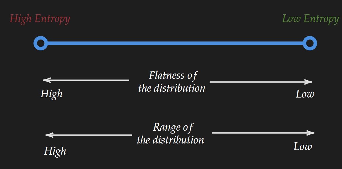
In a nutshell, entropy captures how much uncertainty is associated with a distribution. Now this in turn captures two things: the range of the distribution and the “flatness” of the distribution.

Range of distribution

Let’s describe it with an example. Suppose you are making a 100$ bet. There are two ways to go. One is to make a bet on the distribution for a fair coin toss. You can choose either head or tail. Another is to make a bet on the distribution for a fair die roll. You can choose one out of six possible outcomes. Just from common sense which one would you choose and why?

The answer is pretty obvious. You are going to choose the coin toss. The reason is the distribution range is lower compared to the range of the distribution for a die roll. In other words, there are fewer possible outcomes.

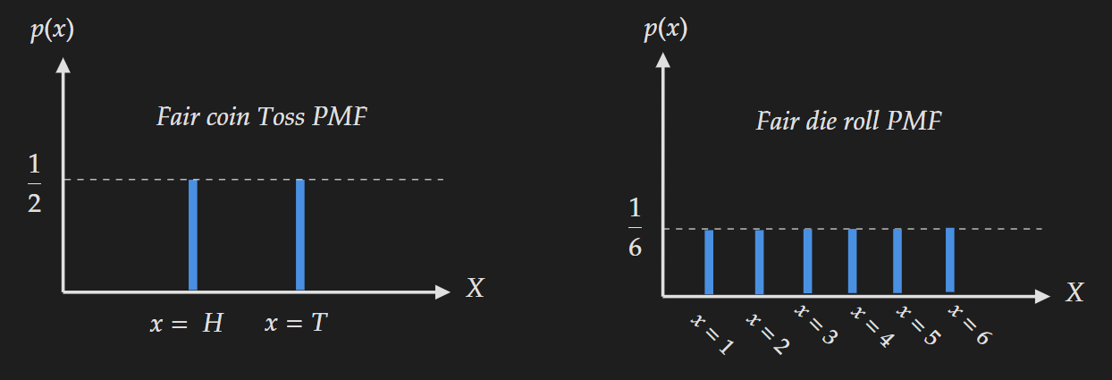
Entropy can capture this “more uncertainty” in the die roll. The larger the range the larger the value of entropy. For the above example with a $\log-e$ base entropy for the coin toss is

\[H_{\text{coin-toss}}(X)=-0.5 \log 0.5-0.5 \log 0.5=0.693\]

But for the die roll entropy is

\[H_{\text{die-roll}}(X)=-6\times\frac{1}{6}\times \log(\frac{1}{6})=1.79\]

which is larger compared to the entropy of the coin toss.

Flatness of Distribution

Let’s take another example to describe how the flatness of distribution is captured by entropy. Suppose you are given a choice to live in two different states. For the two states, the distribution of a day is sunny, rainy, snowy and cloudy looks like below:

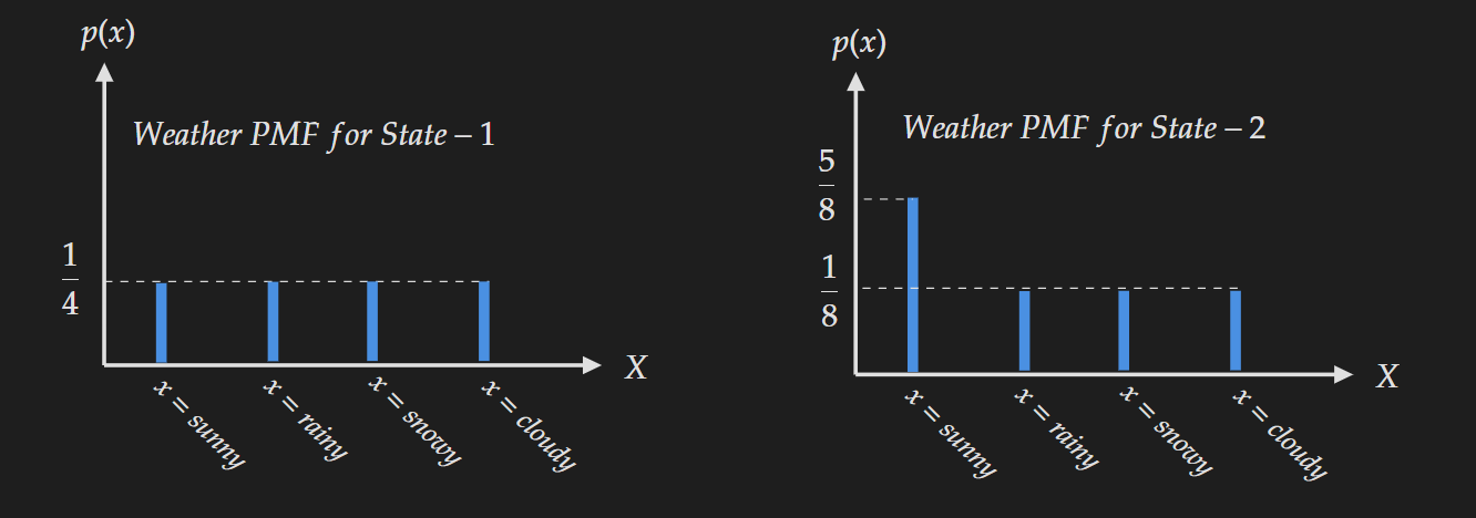
Based on the PMF which state would you choose? If you are like most people you are going to choose “State-2”. The reason is living in “State-1” looks like a nightmare because of the uncertainty in weather. In contrast, the weather for “State-2” is much less uncertain and mostly sunny.

For State-1, the computation of entropy is given below:

\[H_{\text{state-1}}(X)=-4\times\frac{1}{4}\times \log(\frac{1}{4})=1.39\]

For State-2, the computation of entropy is given below:

\[H_{\text{state-2}}(X)=-3\times\frac{1}{8}\times \log(\frac{1}{8})-\frac{5}{8}\times \log(\frac{5}{8})=1.07\]

Entropy can capture this “uncertainty” or “the amount of flatness” in a distribution.

Another such visualization is given below:

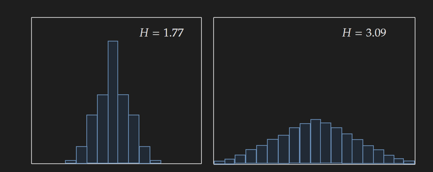Image Adapted from Bishop, C.M. and Nasrabadi, N.M., 2006. Pattern recognition and machine learning

Even though the examples given are for univariate discrete distributions, this core idea is generalized for higher dimensional discrete and continuous distributions. A visual summary is given in the following diagram.