Evidence Lower Bound
Evidence lower bound, commonly known as ELBO is one of the fundamental concepts to understand variational inference and also probabilistic decision theory. I am going to assume that readers are familiar with Bayes Theorem which is a prerequisite concept. If you are not I encourage you to go through some materials like this video. Also, go through my article about Latent Variable Model.
Intractability of Distribution
The main reason to come up with the concept of ELBO (at least originally) is due to the intractability of computing distributions in higher dimensions. In my article about latent variable model I mention the intractability of the following quantity in higher dimensions.
\[p(x)=\int_z p(x \mid z) p(z) d z\]Remember that computing this quantity was a sub-goal, the main goal was to compute the posterior shown in the following equation:
\[p(z \mid x) = \frac{p(x\mid z) p(z)}{\int_z p(x\mid z) \ p(z)}\]If we cannot compute $\int_{z} p(x\mid z) \ p(z)$, then we cannot compute the posterior $p(z \mid x) $. Now rather than trying to compute the exact value for $p(z \mid x)$ we use variational inference to approximate it with another distribution. In this article, I do not want to go deep into variational inference. Hence, the following section gives a small informal introduction to variational inference.
A Hand-Wavy Introduction to Variational Inference
An informal definition of variational inference is that it is a way to approximate a complex distribution with a relatively simpler distribution through the process of optimization. But for optimization, we need a loss function that will tell us how “good” our approximation is. If our approximation is good, we should stop the optimization process. As we are trying to compare between distributions, the obvious loss function that comes to mind is KL Divergence. As KL Divergence quantifies the similarity between two distributions, it can be used as an indicator of how “good” our approximation is. But there is a certain issue with using KL Divergence which is mentioned in the next section. Before we move on to the next section, let’s introduce some terminology and symbols. As I said, the surrogate distribution is a simpler class of distribution we need to explicitly mention the parameters. Assume the exact posterior distribution is $p_{\theta}(z \mid x)$ and the surrogate posterior is $q_{\phi}(z \mid x)$.
The Issue with using KL Divergence as a Loss Function
If we write down the KL Divergence (the reverse KL Divergence) formula between $p_{\theta}(z \mid x)$ and $q_{\phi}(z \mid x)$ we get the following:
\[\begin{aligned} D_{K L}\left(q_\phi(z \mid x) \| p_{\theta}(z \mid x)\right) & =\int_z q_\phi(z \mid x) \log \frac{q_\phi(z \mid x)}{p_{\theta}(z \mid x)} d z \\ \end{aligned}\]Well, calculating this quantity requires knowing the posterior $p_{\theta}(z \mid x)$. This creates a kind of “chicken and egg” problem. The work-around is getting an expression for ELBO which is shown in the next section.
Derivation of ELBO
\[\begin{aligned} D_{K L}\left(q_\phi(z \mid x) \| p_{\theta}(z \mid x)\right) & =\int_z q_\phi(z \mid x) \log \frac{q_\phi(z \mid x)}{p_{\theta}(z \mid x)} d z \\ & =-\int_z q_\phi(z \mid x) \log \frac{p_{\theta}(z \mid x)}{q_\phi(z \mid x)} d z \\ \end{aligned}\]Now we can replace $p_{\theta}(z \mid x)$ with following quantity,
\[p_{\theta}(z \mid x) = \frac{p_{\theta}(x,z)}{p_{\theta}(x)}\]After replacing we get the following:
\[\begin{aligned} D_{K L}\left(q_\phi(z \mid x) \| p_{\theta}(z \mid x)\right) & =-\int_z q_\phi(z \mid x) \log \frac{p_{\theta}(x, z)}{q_\phi(z \mid x) p_{\theta}(x)} d z \\ & =-\left(\int_z q_\phi(z \mid x) \log \frac{p_{\theta}(x, z)}{q_\phi(z \mid x)} d z-\int_z q_\phi(z \mid x) \log p_{\theta}(x) d z\right) \\ & =-\int_z q_\phi(z \mid x) \log \frac{p_{\theta}(x, z)}{q_\phi(z \mid x)} d z+ \boxed{\log p_{\theta}(x)} \end{aligned}\]Notice that we have the quantity $\log p_{\theta}(x)$ in our expression which is the log evidence. Now we can rewrite it as below:-
\[\log p_{\theta}(x) = \int_z q_\phi(z \mid x) \log \frac{p_{\theta}(x, z)}{q_\phi(z \mid x)} d z + D_{K L}\left(q_\phi(z \mid x) \| p_{\theta}(z \mid x)\right)\]Now we know that KL Divergence is a non-negative quantity ( a simple proof is available in Jensen’s Inequality article) which means $D_{K L}\left(q_\phi(z \mid x) | p_{\theta}(z \mid x)\right) \geq 0$.
This means we can set a lower bound on $\log p_{\theta}(x)$. The possible lowest value it can acquire when $D_{K L}\left(q_\phi(z \mid x) | p_{\theta}(z \mid x)\right) = 0$ and that case $\log p_{\theta}(x) = \int_z q_\phi(z \mid x) \log \frac{p_{\theta}(z, x)}{q_\phi(z \mid x)} d z $
Therefore we can write the following,
\[\log p_{\theta}(x) \geq \int_z q_\phi(z \mid x) \log \frac{p_{\theta}(x, z)}{q_\phi(z \mid x)} d z\]This is the reason behind naming this quantity evidence lower bound as it imposes a lower bound on the log-evidence. Now if we maximize this quantity that in turn will mean minimizing $D_{K L}\left(q_\phi(z \mid x) | p_{\theta}(z \mid x)\right) $ which was our original goal.
\[\log p_{\theta}(x) =\underbrace{\int_z q_\phi(z \mid x) \log \frac{p_{\theta}(x, z)}{q_\phi(z \mid x)} d z }_{\text{Maximizing ELBO means}}+ \underbrace{D_{K L}\left(q_\phi(z \mid x) \| p_{\theta}(z \mid x)\right)}_{\text{Minimizing this}}\]So, the mathematical expression of ELBO is given below:
\[\begin{align*} \text{ELBO} &=\int_z q_\phi(z \mid x) \log \frac{p_{\theta}(x, z)}{q_\phi(z \mid x)} d z \\ &= \int_{z}q_\phi(z \mid x) \log p_{\theta}(x, z) dz - \int_{z}q_\phi(z \mid x) \log q_{\phi}(z \mid x) dz \\ & = \mathbb{E}_{q_{\phi}(z|x)}[\log p_{\theta}(x, z)] -\mathbb{E}_{q_{\phi}(z|x)}[\log q_{\phi}(z \mid x)] \end{align*}\]We can further simplify this as shown below:
\[\begin{align*} \text{ELBO} & = \mathbb{E}_{q_{\phi}(z|x)}[\log p_{\theta}(x, z)] -\mathbb{E}_{q_{\phi}(z|x)}[\log q_{\phi}(z \mid x)]\\ & =\mathbb{E}_{q_{\phi}(z|x)}[\log (p_{\theta}(x \mid z)\times p_{\theta}(z))]-\mathbb{E}_{q_{\phi}(z|x)}[\log q_{\phi}(z \mid x)] \\ &= \mathbb{E}_{q_{\phi}(z|x)}[\log p_{\theta}(x \mid z)] +\mathbb{E}_{q_{\phi}(z|x)}[\log p_{\theta}(z)]-\mathbb{E}_{q_{\phi}(z|x)}[\log q_{\phi}(z \mid x)] \\ & = \underbrace{\mathbb{E}_{q_{\phi}(z|x)}[\log p_{\theta}(x \mid z)]}_{\text{Expected log-likelihood}}- \underbrace{D_{KL}(q_{\phi}(z|x) \| p_{\theta}(z))}_{\text{KL Divergence between prior and surrogate}} \\ \end{align*}\]This means when we try to maximize ELBO we are essentially trying to maximize the expected log-likelihood and minimize the KL Divergence between the prior and the surrograte.
ELBO is expressed with the symbol $\mathcal{L}$ and we can write the objective as $ \underset{q} {\max}~\mathcal{L}$ i.e. maximization of ELBO.
Connection to VAE
So far we have been talking about ELBO with any specific application in mind. Variational Autoencoder uses the concept of ELBO.
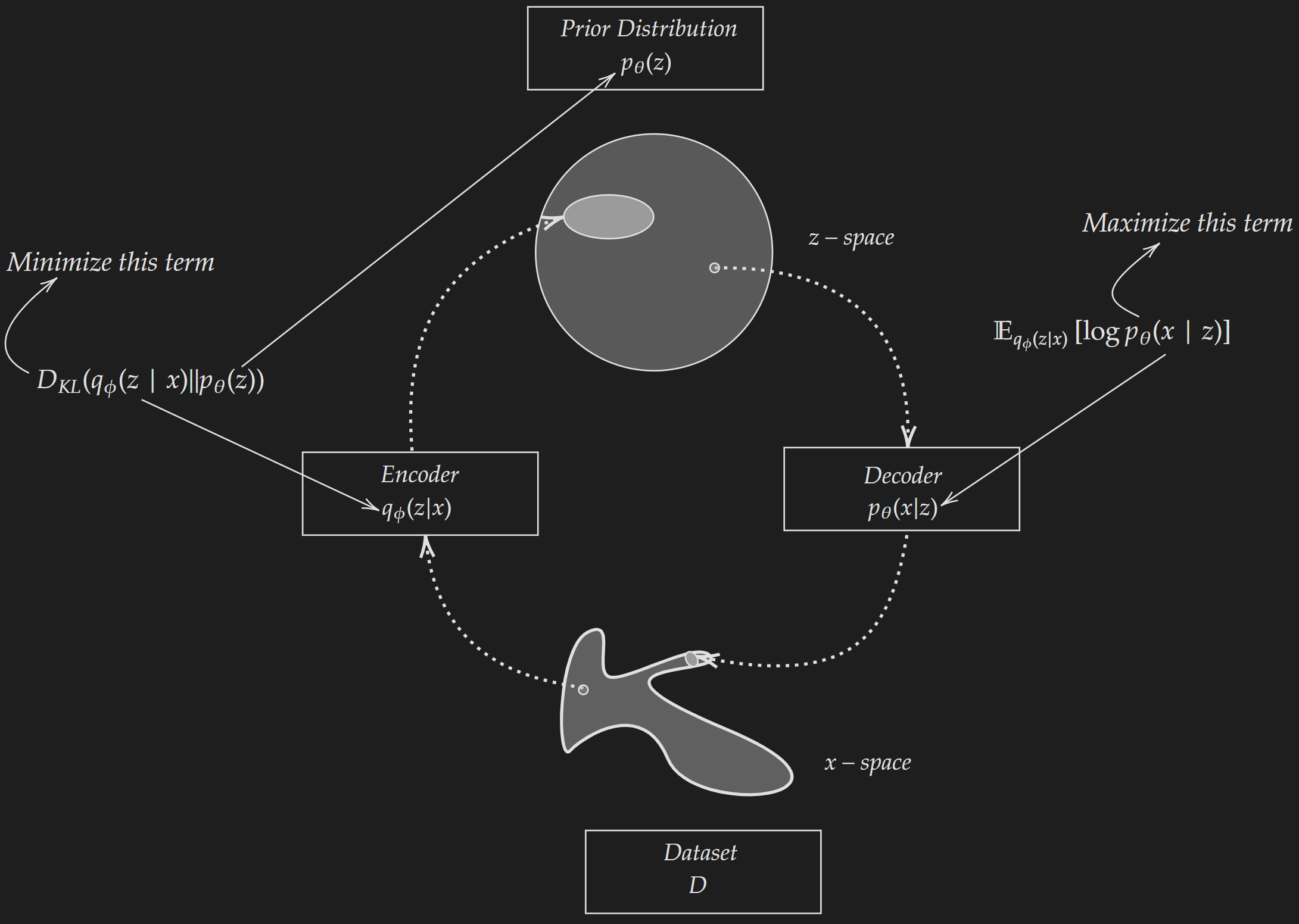 Image Adapted from Kingma, Diederik P., and Max Welling. “Auto-encoding variational bayes”