A Reference Guide to Statistics
This article acts as a repository of the concepts I learned about any topics in Statistics. I plan to use this as a reference for ideas/concepts/formulas in Statistics. Essentially this is a look-up reference guide; if I forget any specific topic, I can revise that topic again. A significant portion of these concepts is based on the videos from the following YouTube channels.
In addition, several blog posts and texts are also used as references.
Inferential Statistics
Sampling
References: Sampling Distributions (7.2)
A sample is a small portion of the population that we examine and draw conclusions from.
The process of drawing a sample from the population is known as sampling.
Sample Distribution
When we draw a particular sample from a distribution, that specific sample creates a distribution. This is known as the “sample distribution”.
Sampling Distribution
The sampling distribution of a statistic is the probability distribution of that statistic. This means if we draw samples from the population a bunch of times, the distribution associated with a particular statistic is referred to as the sampling distribution.
The sample statistic is known as the point estimate of the population parameter.
Sampling Distribution of the Sample Mean
References: Sampling Distributions (7.2), The Sampling Distribution of the Sample Mean
For example, let’s use “mean” as the statistic. In that case, given a population (say all people in Wisconsin) and a random variable (say weight) we have a “true” population distribution of people’s weights. Now we draw a sample from that distribution to calculate the mean weight for that sample and plot it into a histogram. We do this process again and again. The resulting histogram generated from this is the mean sampling distribution. Think of the sample mean $\bar{X}$ as a random variable. Depending on which sample we choose it changes, therefore that is variable and randomness comes from the sampling process and the size of the sample. One fact is that this sampling distribution approaches a normal distribution due to the central limit theorem (under certain conditions). Three key facts about the sample mean given the sample size equals $n$:
The expected value of the sample mean $\bar{X}$ equals the population mean meaning $\mathbb{E}(\bar{X})=\mu_{\bar{X}}=\mu$.
The variance value of the sample mean $Var(\bar{X})=\frac{\sigma^{2}}{n}$.
The standard error of the sample mean equals the population standard deviation divided by the square root of the sample size; $se(\bar{X})=\sigma_{\bar{X}}=\frac{\sigma}{\sqrt{n}}$.
Other two key facts:
If the original population distribution is normally distributed, then the sampling distribution will also be a normal distribution with sample mean equals $\mu$ and standard error equals $\frac{\sigma}{\sqrt{n}}$ i.e. $\bar{X} \sim \mathcal{N}(\mu,\frac{\sigma^{2}}{n})$
If the original population distribution is not normally distributed, the sampling distribution might approach the normal distribution due to the central limit theorem but the sample size needs to be large enough for the normal approximation to be reasonable. In practice, the sample size needs to be $n\geq30$.
We can standardize the sampling distribution of the sample mean as follows:-
\[Z= \frac{\bar{X}-\mu}{\frac{\sigma}{\sqrt{n}}}\]This will result in a standard normal distribution.
Sampling Distribution of the Sample Proportion
References: The Sampling Distribution of the Sample Proportion
Here the statistic we are interested in is the proportion.
The sampling distribution of the sample proportion is closely related with the binomial distribution.
Three key facts about the sample proportion given the sample size equals $n$:
The expected value of the sample proportion $\bar{p}$ (this is sometimes denoted as $\hat{p}$) is equal to the population proportion; that is $\mathbb{E}(\bar{p})=\frac{X}{n}=p$.
The variance value of the sample proportion $Var(\bar{p})=\frac{p(1-p)}{n}$.
The standard error of the sample proportion $\bar{p}$ equals $se(\bar{p})=\sqrt{\frac{p(1-p)}{p}}$
One other key fact:
- For any population proportion $p$, the sampling distribution of $\bar{p}$ is approximately normal if the sample size $n$ is sufficiently large enough, As a general guideline $np \geq 5$ and $n(1-p)\geq 5$. However, this guideline is different in different references.
Sampling Distribution of the Sample Variance
References: The Sampling Distribution of the Sample Variance
Let’s start by defining the sample variance. Mathematically, the sample variance denoted as $s^2$ can be defined as follows:
\[s^2=\frac{\sum\left(X_i-\bar{X}\right)^2}{n-1}\]with sample variance, we are trying to get the point estimate of the population parameter which is variance $\sigma^2$.
If we compute this sample variance numerous times and take the expectation, in the long learn we are going to get the population variance $\sigma^2$.
\[E\left(s^2\right)=\sigma^2\]What factors determine the sampling distribution of the sample variance:
- Which distribution we are sampling from
- The sample size $n$
Sampling Distribution of the Sample Variance for a normal distribution
Suppose the distribution we are sampling from is normally distributed with a population variance of $\sigma^2$. And we sample $n$ independent samples from the distribution. In that case, the sampling distribution of modified sample variance (modified by scaling with $\frac{(n-1)}{\sigma^2}$) is given by a chi-square distribution which can be expressed as follows:
\[\chi^2=\frac{(n-1) s^2}{\sigma^2}\]This is chi-square distribution with $n-1$ degrees of freedom. Again to reiterate this is not the exact distribution for the sample variance; rather a scaled version of the sample variance. Sometimes the expression is modified and written as follows to explicitly mention the degrees of freedom:
\[\chi_{n-1}^2=\frac{(n-1) s^2}{\sigma^2}\]For low sample size the distribution is skewed. As the sample size increases the distribution becomes more and more symmetric.
t-Distribution
References: Introduction to the t Distribution (non-technical), What is the t-distribution? An extensive guide!
Interactive Visualization: Kristoffer Magnusson
One issue when working with the sampling distribution of the sample mean is for many calculations we are required to know $\sigma$. But $\sigma$ is a population parameter which is most of the time not possible to know. This means we can not calculate the following quantity as $\sigma$ is unknown:
\[Z= \frac{\bar{X}-\mu}{\frac{\sigma}{\sqrt{n}}}\]The solution is to use $s$ which is the sample standard deviation instead of $\sigma$. But $s$ is not a constant in contrast to $\sigma$. As a result, the following quantity is no longer a standard normal distribution:
\[T=\frac{\bar{X}-\mu}{s / \sqrt{n}}\]Here, $T$ is a random variable which follows the t-distribution. It is characterized by degrees of freedom where for the above equation the degree of freedom equals $n-1$.
Comparison with Normal Distribution
Both t-distribution and standard normal distribution are bell-shaped and symmetric about $0$, but t-distribution has broader tails. The reason is for standard normal distribution we work with population parameters that are constant. This implies less variability. But for t-distribution, we replace $\sigma$ with $s$ which is a statistic, not a population parameter. This increases the variability of the distribution hence broader tails.
The fewer the degrees of freedom the broader the tails.
Confidence Interval
References: Introduction to Confidence Intervals, What are confidence intervals? Actually. , Confidence Intervals - Introduction
Interactive Visualization of Confidence Interval: From Seeing theory, By Kristoffer Magnusson
A confidence interval is a range of values that is constructed around a sample statistic, such as a mean or a proportion, to estimate the true population parameter with a certain level of confidence.
Sometimes known as interval estimate in contrast to point estimate.
For further clarification, another definition is given below:
A confidence interval, or interval estimate, provides a range of values that, with a certain level of confidence, contains the population parameter of interest.
Now one really important thing to keep in mind, the interval estimate or the confidence interval is for the population parameter. We are not trying to get an interval estimate for sample statistics.
The core idea is conveyed by the following equation:
\[\boxed{\text{Point Estimate} \ \pm \ \text{Margin of Error}}\]Confidence Interval for Population Mean $\mu$
When the population standard deviation is known
A (1-$\alpha$)$\times 100\%$ confidence interval for $\mu$
\[\boxed{\bar{X} \pm z_{\alpha / 2} \times \frac{\sigma}{\sqrt{n}}}\]where,
- $\bar{X}$ is the sample mean
- $\sigma$ is the population standard deviation. In practice, this is rarely known.
- $n$ sample size
- $\frac{\sigma}{\sqrt{n}}$ is the standard error of the sampling distribution i.e. $se(\bar{X})=\sigma_{\bar{X}}$
- $z_{\alpha /2}$ is the z-value determined based on the value of $\alpha$
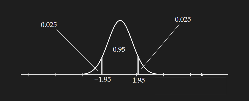 Visualization for 95% confidence interval
For $(1-\alpha)\times 100\%=95\%$ confidence interval the value of $\alpha=5\% =0.05$. Based on this $\frac{\alpha}{2}=0.025$. We can use software or the standard normal table to determine the $z_{\alpha/2}=z_{0.025}$.
When the population standard deviation is not known
\[\boxed{\bar{X} \pm t_{\alpha / 2, \nu} \frac{s}{\sqrt{n}}}\]where,
- $\bar{X}$ is the sample mean
- $s$ is the sample standard deviation.
$n$ sample size
$t_{\alpha / 2, \nu}$ is the critical value from t-distribution which is dependent on both $\alpha$ and $\nu$.
- $\nu$ is the degrees of freedom of the t-distribution which is equal to $n-1$
Note that with a larger sample size of $n$, the quantity $t_{\alpha / 2, \nu} \frac{s}{\sqrt{n}}$ decreases. This implies with a large sample size, our confidence interval is more tight.
Confidence Interval for Population Proportion $p$
A $(1-\alpha)\times 100\%$ confidence interval for $p$
\[\hat{p}\pm z_{\alpha / 2} \sqrt{\frac{\hat{p}(1-\hat{p})}{n}}\]Sometimes it is written in terms of standard error as follows:
\[\hat{p} \pm z_{\alpha / 2} ~S E(\hat{p})\]Here,
- $\hat{p}$ is the sample proportion
- $ z_{\alpha / 2}$ is a critical value which is dependent on $\alpha/2$
- $S E(\hat{p})$ is the standard error for sample proportion
Hypothesis Testing
First, let’s try to understand what we mean by “Hypothesis”. This kind of a general term to refer to a “claim” or a premise. We perform tests to check the “Hypothesis” hence the name “hypothesis testing”. Now, this might seem ambiguous because of how general the definition is. That is an unfortunate consequence of trying to avoid attaching a concept to a specific example. Sometimes the concept seems way too abstract.
Null hypothesis:
This is denoted as $H_0$. This is the accepted value (for now) for a parameter. Again, we are ambiguous about what we mean by a “parameter”. Again, the reason is we want it to be general. The parameter can be a mean or a proportion or predicted coefficients of the regression model…..
Alternative hypothesis:
This is denoted as $H_a$
There are two possible outcomes from hypothesis testing:
- We can reject the null hypothesis.
- Or we can fail to reject the null hypothesis. Note that, we did not prove the “null hypothesis” is actually true.
A good analogy for this is “You are innocent until proven guilty”. Using that analogy we can say “Null hypothesis is true unless the evidence we get is substantial enough to accept the alternative hypothesis and reject the null hypothesis”. Well, we need to define and quantify what we mean by “substantial evidence”.
Defining substantial evidence: We use test statistics (the statistic for the parameter) to get the “evidence”. Note that, this is “statistic” because we will always be working with samples. Also, this indicates what we mean by “substantial evidence”. Because when we work with “statistics” and get a sampling distribution for a parameter, there is always randomness. So, by “substantial evidence” we mean we can say without any doubt the evidence against the null hypothesis did not happen because of randomness. Let’s test a concrete example, assume we make a null hypothesis about the weight of people in Wisconsin. The null hypothesis is: The proportion of people that are overweight in Wisconsin is 0.3. And the alternative hypothesis is: The proportion of people who are overweight in Wisconsin is not 0.3.
\[H_0: \text{Proportion of overweight people in Wisconsin }=~0.3\] \[H_a: \text{Proportion of overweight people in Wisconsin is}\neq~0.3\]Well, to get evidence to reject the null hypothesis, we collect a sample and measure the proportion of people who are overweight. Say, that comes out to be $0.32$. Does that mean we should reject the null hypothesis? Obviously not, because that small deviation can happen by random chance. We need some really extreme evidence to reject the null hypothesis. This is where things become fuzzy and subjective. We need to quantify exactly what evidence would convince us to reject the null hypothesis.
One-tailed vs Two-tailed test:
Let’s rewrite the statements for hypothesis testing again but in a concise manner:
Two-tailed test: In two-tailed test, typically the alternative hypothesis statement involves a $\neq$ symbol and the null hypothesis involves an equal symbol.
\[H_0: p=~0.3\] \[H_a: p \neq~0.3\]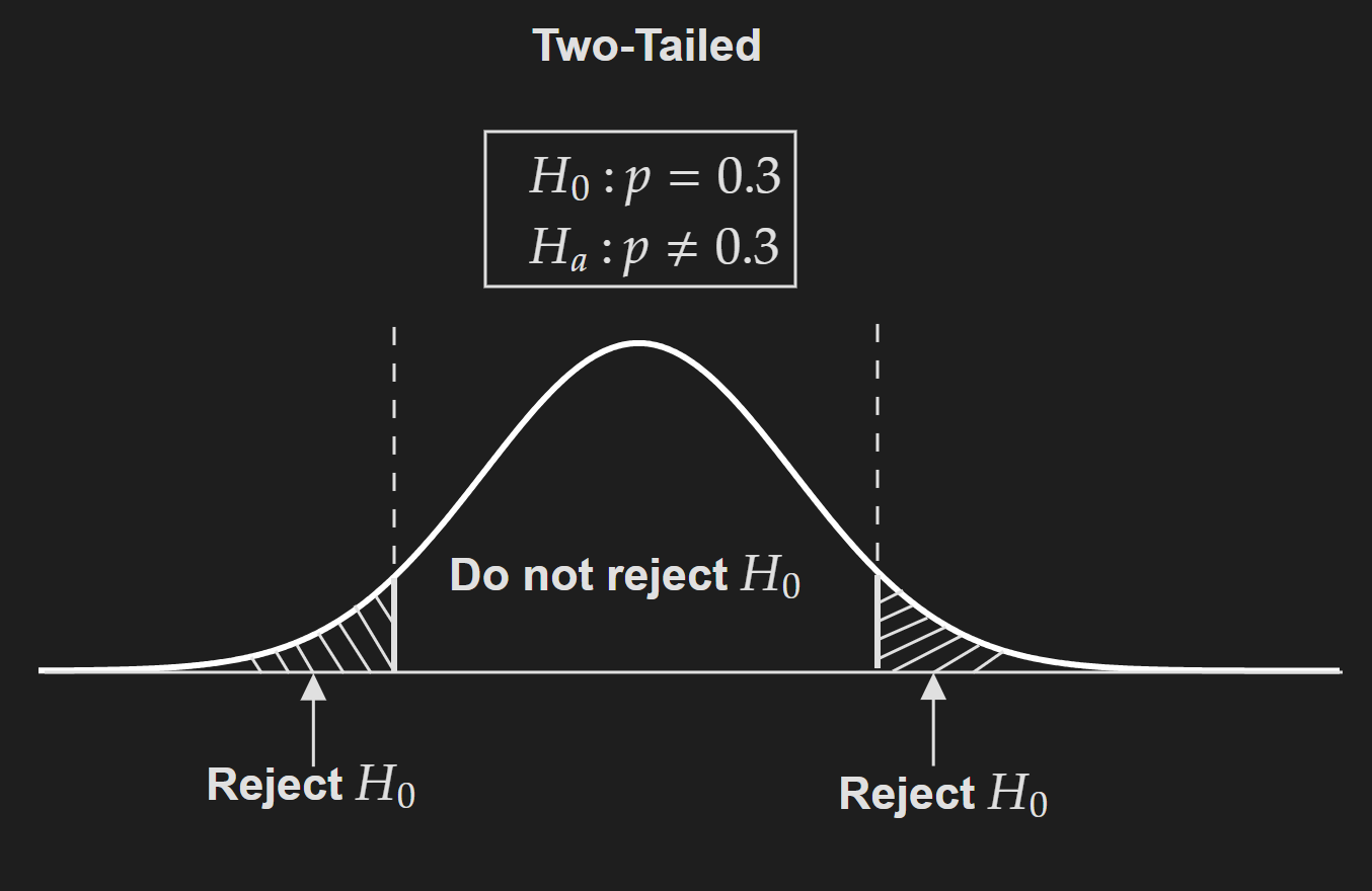
Two-tailed test is sometimes referred to as non-directional hypothesis testing
Process of performing a two-tailed hypothesis test:
Decide on the null hypothesis ($H_0$) and the alternative hypothesis ($H_a$).
Decide on the confidence level ($(1-\alpha)\times 100\%$) or the level of significance value ($\alpha$). The most common value for the confidence level is $95\%$, which means the overall level of significance is $\alpha=0.05$. But as we are doing a two-tailed test we need to compute $\alpha/2=0.025$ for two tails.
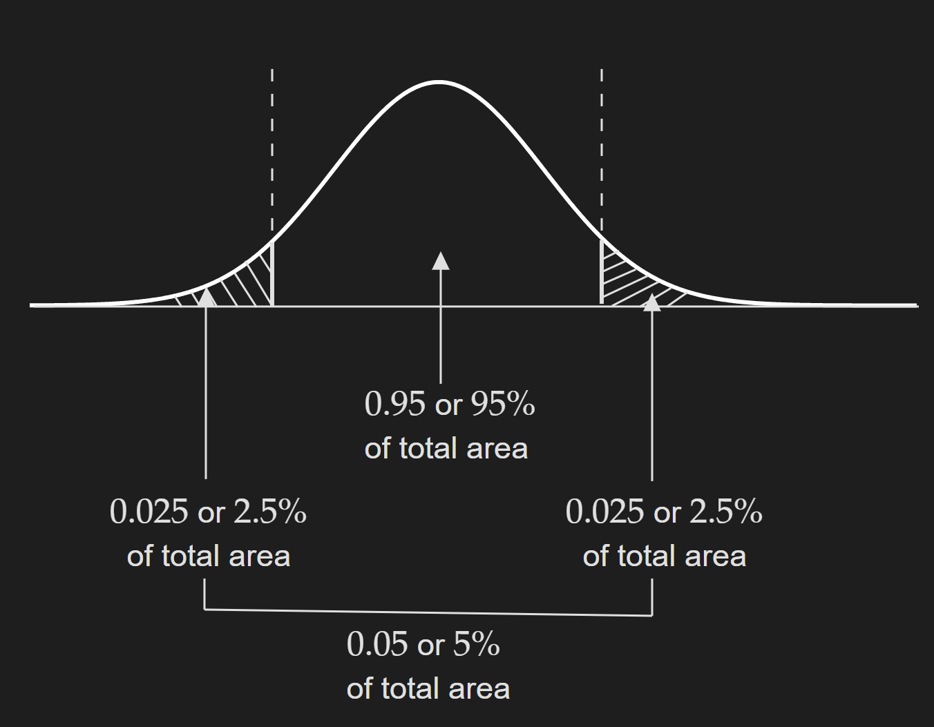
Note that this is going to change if we change our confidence level or level of significance. There is no general rule for choosing this; rather it depends on the domain. For example, if you are doing something in the medical domain, your level of confidence should be pretty high. There are other nuances to decide on this but they are specific to specific cases.
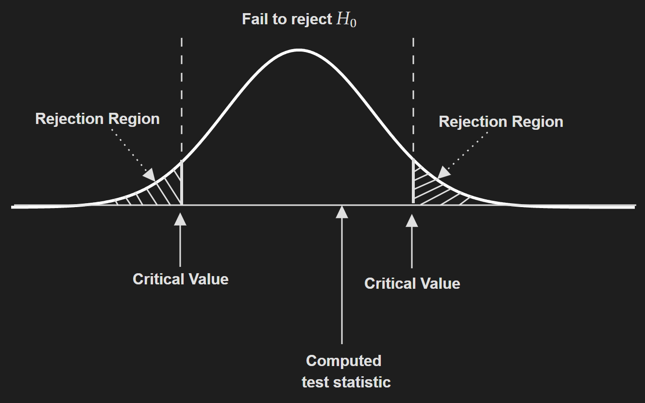
Then we need to compute the critical value. But this is dependent on which statistic we are working with. For example, if we are working with z-statistic and by hypothesis testing we are trying to evaluate an assumption about a population mean then the critical value is typically $1.96$. In short, this is not that straightforward and depends on a lot of factors. Take a look at this cheatsheet to get a feeling for this.
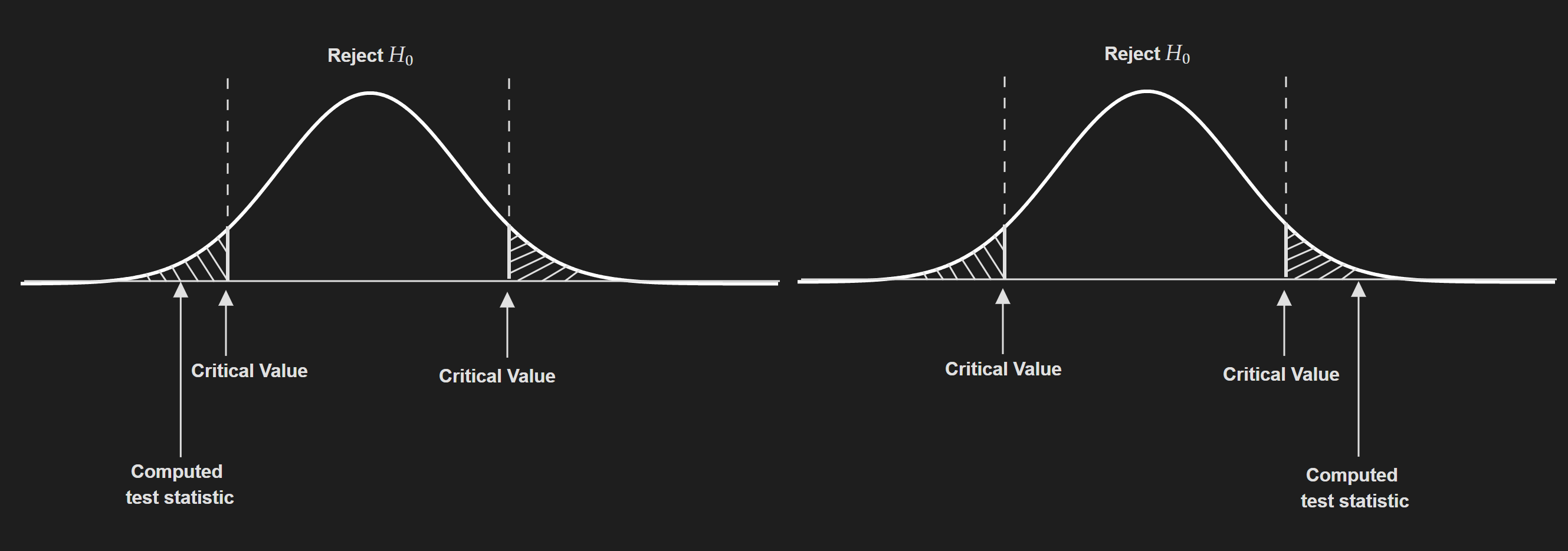
Compute test statistic based on the data and compare it to the critical value.
If the absolute value of the test statistic is greater than the critical value, you reject the null hypothesis. Otherwise, you say we fail to reject the null hypothesis.
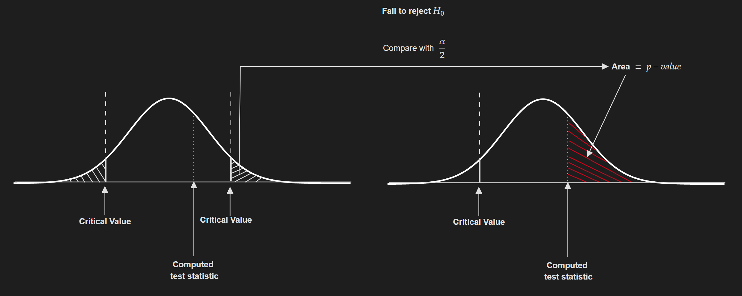
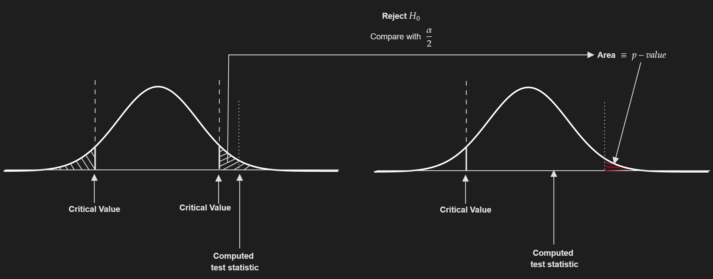
- Another way to do this is using the concept of p-value. The general rule is:
If $p$-value $\leq \alpha / 2$: Reject the null hypothesis.
If $p$-value $>\alpha / 2$: Fail to reject the null hypothesis.
One-tailed test:
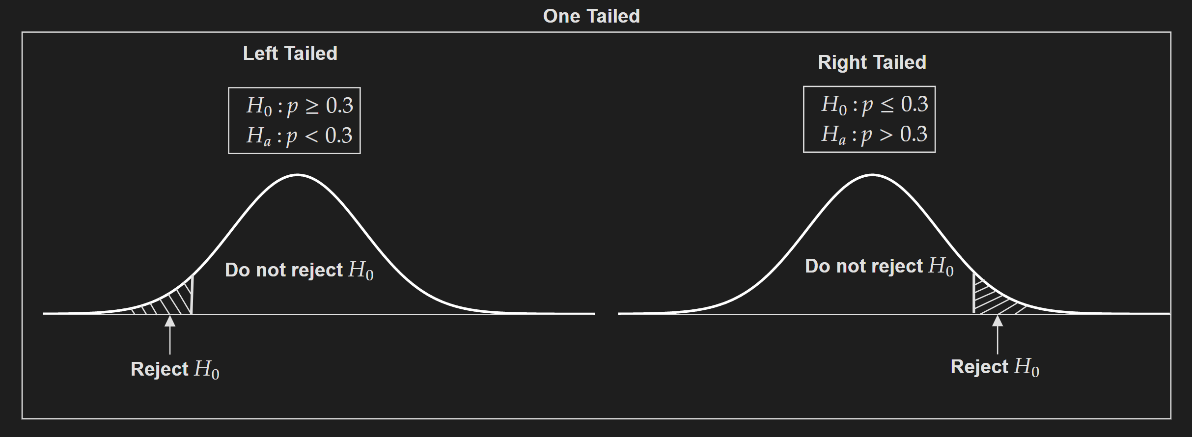
Left-tailed test (Version 1):
\[H_0: p\geq~0.3\] \[H_a: p <~0.3\]Left-tailed test (Version 2):
\[H_0: p =~0.3\] \[H_a: p <~0.3\]Right-tailed test (Version 1):
\[H_0: p\leq~0.3\] \[H_a: p > ~0.3\]Right-tailed test (Version 2):
\[H_0: p=~0.3\] \[H_a: p > ~0.3\]Left-tailed test and right-tailed test are sometimes referred to as directional hypothesis testing
p-value
Reference: What is a p-value? P Values, z Scores, Alpha, Critical Values
Definition: The p-value is the probability of getting the observed value of the test statistic or a value with even greater evidence against $H_0$, if the null hypothesis is true.
Facts about p-values:
- p-value is a probability.
- When we compute the p-value we are assuming the null hypothesis is true.
When the p-values start to go low we start to doubt the null hypothesis. In other words, we start to get uncomfortable about the null hypothesis. We set a threshold (usually 0.05) and when p-value goes down below that threshold we reject the null hypothesis.
- If the p-value does not go down below the threshold we cannot reject the null hypothesis. In other words, the evidence we get to reject the null hypothesis is not statistically significant enough.
Resampling techniques
Resampling techniques are usually used to compute different versions of the training dataset. These different versions of the training dataset can be used to refit a model again and again to gain additional insights and information.
Bootstrapping
Interactive Visualization : From Seeing Theory
Before understanding the concept of bootstrapping, we need to understand why we even need bootstrapping.
The motivation behind bootstrapping: In statistics, we try to estimate a population parameter. But the population is unobservable in practice, hence we work with a sampling distribution and try to estimate the population parameter from the sampling distribution. But to construct a sampling distribution we need to have certain assumptions:
We can take multiple samples from the distribution and compute a statistic for each sample. Taking multiple samples allows us to construct the sampling distribution and do stuff like creating a confidence interval from the sampling distribution.
Another important assumption is the underlying population is Gaussian. If it is not, the sample size is large enough for the central limit theorem to kick in.
What if these assumptions are violated? What if you have a single sample?
Issues: For a single sample, the statistic computed from that sample will be closer to the actual population parameter if the sample size is really large. If the sample size is small, it will to far off from the actual population parameter. In addition, with a single sample, how do you create a confidence interval?
Bootstrapping tries to solve these issues by using a resampling technique. Note that it is a generalized technique that is applicable to any population parameter, like population mean, population proportion, regression coefficients, etc.
See the following visualization that I created as part of a class activity for the Statistical Machine Learning course at Marquette University.
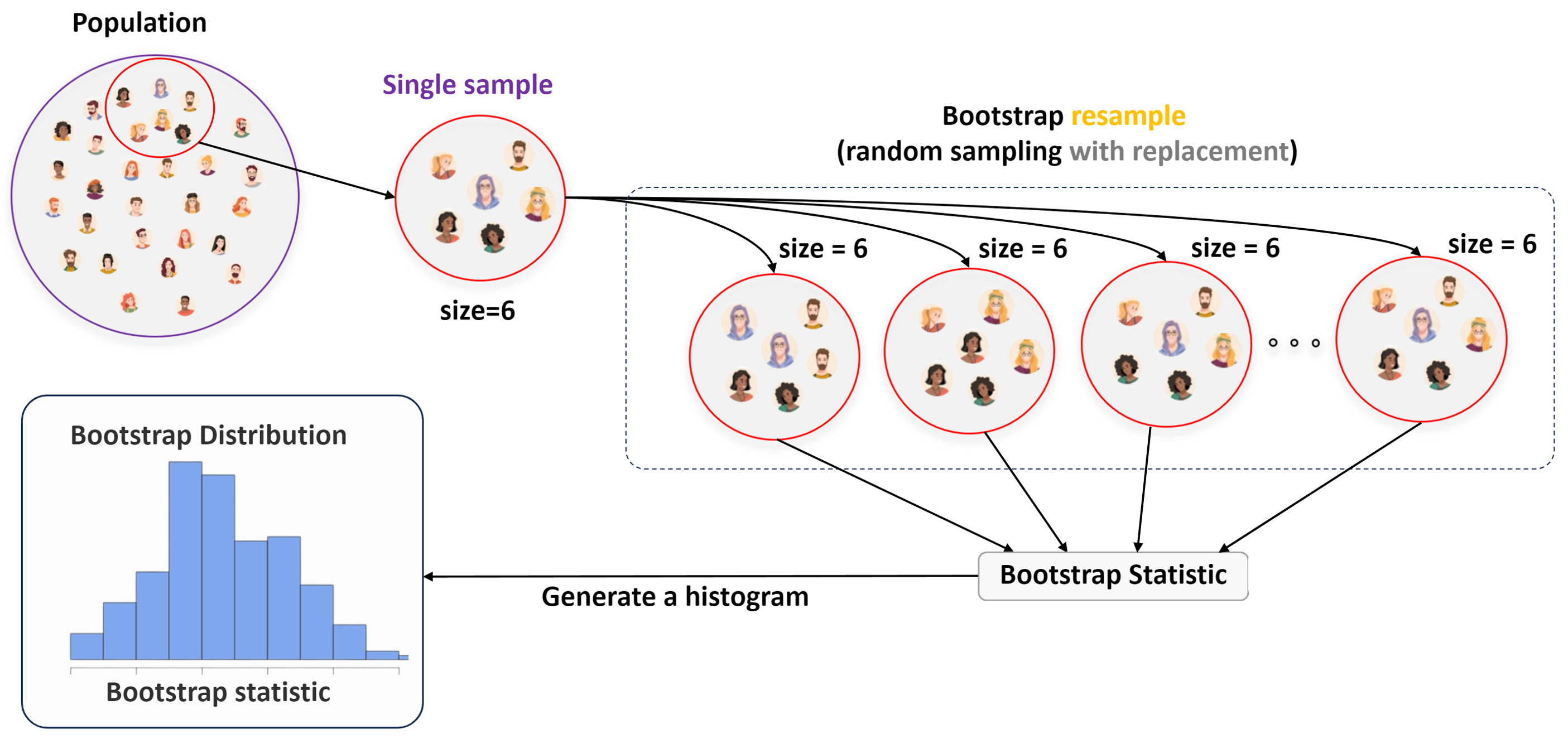
Resample with replacement and create a bootstrapped dataset
Using the bootstrapped dataset compute a statistic.
Generate the bootstrap distribution
This distribution is a non-parametric estimation of the population. This can be used to compute standard error and form confidence intervals.
See the following code example in R. This was also part of the class activity for the Statistical Machne Learning course in Marquette.
1
2
3
4
5
6
7
8
9
10
11
12
13
14
15
16
17
18
19
20
21
22
23
24
25
26
27
28
29
30
31
32
33
34
35
36
37
38
39
40
41
42
43
44
45
46
47
48
49
50
51
52
53
54
55
# Import the packages
library(infer)
library(ggplot2)
library(dplyr)

# Set Random seed
set.seed(6520)

# Load the built in gss dataset
data(gss)

# Take a look at the population dataset
dplyr::glimpse(gss)

# Find the population mean
population_mean <- mean(gss$hours)

# Randomly choose 20 row indices from the original dataframe
random_indices <- sample(nrow(gss), 20)

# Subset the original dataframe using the randomly chosen indices
sample_dataset<- gss[random_indices, ]

# Take a look at the sample dataset
dplyr::glimpse(sample_dataset)

# Finding the mean with Bootstrapping
boot_dist <- sample_dataset %>%
  specify(response = hours) %>%
  generate(reps = 1000, type = "bootstrap") %>%
  calculate(stat = "mean")

# Visualize bootstrap distribution
boot_dist %>%
  visualize()+
  theme_bw()

# Form the confidence interval
ci <- infer::get_ci(
  boot_dist, level = .95)

# Compute the sample mean
obs_mean <- sample_dataset %>%
  specify(response = hours) %>%
  calculate(stat = "mean")

# Visualise
boot_dist %>%
  visualize() +
  shade_confidence_interval(endpoints = ci)+
  geom_vline(xintercept = population_mean,
             color = "red",linetype = "dashed",size = 3)+
  geom_vline(xintercept = obs_mean[[1]],
             color = "blue",size = 3)+
  theme_bw()
Let’s also talk about some of the limitations of the bootstrap method.
It is computationally expensive which is obvious.
Bootstrap cannot fix a bad sample that is not representative of the population.
If the sample size is too small bootstrap cannot fix that.
Bootstrap does not do anything for bias correction.
Cross-validation
There are different variations of the cross-validation approach. The most well-known ones are K-fold cross-validation and Leave-one-out cross-validation (LOOCV). However, blindly using these techniques without considering different assumptions can reach to wrong conclusions. For example in case of a classification problem, if your dataset is severely imbalanced stratified K-fold should be used rather than vanilla K-fold cross-validation. Interested readers should look into Sckit-learn documentation which provides API for the following cross-validation methods:
- K-fold
- Repeated K-Fold
- Leave One Out
- Leave P Out
- Stratified k-fold
- Stratified Shuffle Split
- Group k-fold
- StratifiedGroupKFold
- Leave One Group Out
- Leave P Groups Out
- Group Shuffle Split
I think the Sckit-learn documentation does a pretty good job of explaining them, so I won’t go into too much detail.
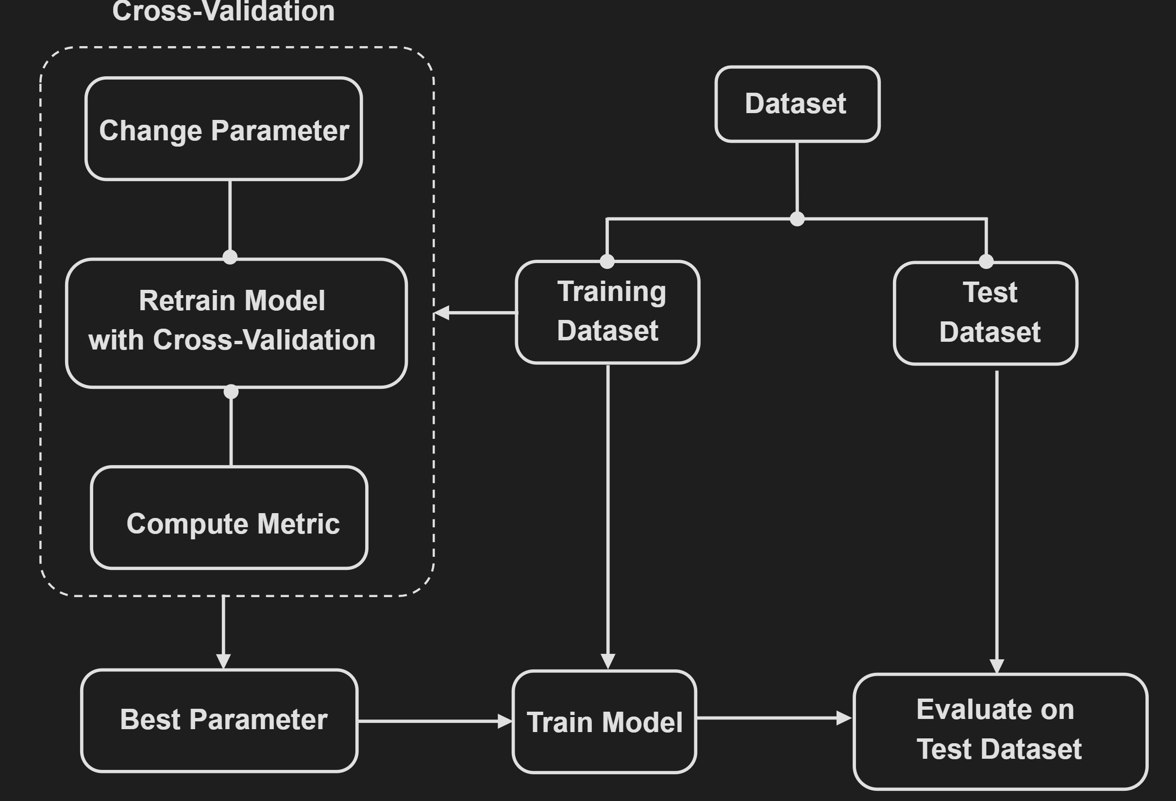
One use case of cross-validation is choosing (hyper)parameters. The following diagram visualizes this process:
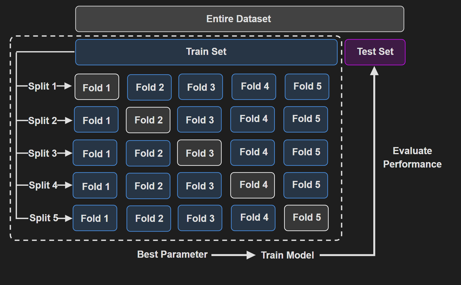
Another visualization that shows $5$-fold cross validation :
It is easily apparent that CV increases the computational cost significantly. If you ever used GridSearchCV for choosing hyperparameters, you will understand what I am talking about. If the number of (hyper)parameters is low, then it is kind of manageable. But as the number increases the computational complexity quickly gets out of hand.
Another use case is providing a robust estimate of the model performance. When we perform a single train-test split, there’s a risk that the split might not be representative of the overall dataset. Cross-validation helps mitigate the variability of test splits by systematically cycling through different train-test splits, providing a more robust estimate of model performance.
References
[1] Jaggia, S., Kelly, A., Lertwachara, K. and Chen, L., 2021. Business analytics: Communicating with numbers. McGraw-Hill Education.