A Reference Guide to Distributions
I know it is dumb to create a reference guide to distributions because it is too large of a topic to keep a reference on. I mean there are entire books written on these distributions. Also, some distributions are domain-specific. For example, an engineer who works with the applications of wireless communication will surely know about Rayleigh and Rician distributions. Hence, it is kind of a waste of energy and time to try to learn about all the distributions. But still, I want to keep a reference of distributions I come across often when going through literature. Interestingly, most of the distributions come from the exponential family.
Additionally, I want to mention some external resources that provide interactive visualizations of probability distributions.
⦿ Discrete Probability Distributions
⯈ Bernoulli Distribution
The best way to think about this distribution is to think about a biased coin toss where the probability of a head is $p$ and the probability of a tail is $1-p$. Whenever I come across any scenario that involves Bernoulli distribution, I try to project that scenario into a biased contain toss.
⯌ Probability Density Function:
The compact form of distribution looks scary and unintuitive (the first one below) and throws people off. The more intuitive one is the second one which shows the distribution is parameterized by a single probability value $p$. \(\begin{align*} \operatorname{P}(X=x \mid p) &=p^{x}(1-p)^{1-x} \\ &= \begin{cases}p & x=1 \\ 1-p & x=0\end{cases} \end{align*}\)
\[\text { where, } p \in[0, 1]\]Here,
- $p$ is the probability of success and $(1-p)$ is the probability of failure
- $x=1$ defines the success event and $x=0$ defines the failure event
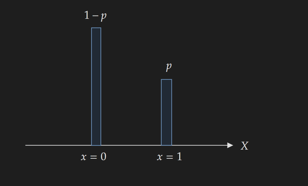 The PMF is completely determined by the value of $p$
⯌ Cumulative Density Function:
\[\operatorname{P}(X\leq x )=\begin{cases}0 & \text { if } x<0 \\ 1-p & \text { if } 0 \leq x<1 \\ 1 & \text { if } x \geq 1\end{cases}\]⯌ Expected Value:
\[\boxed{E(X)=p}\]⯌ Variance:
\[\boxed{Var(x)=p(1-p)}\]⯌ Properties and Key Facts:
- The number of trials is equal to $1$.
- Model events when there are only two possible outcomes: success and failure.
- It is a special case of binomial distribution where number of trials $n=1$
- Binomial distribution, Negative Binomial Distribution and Geometric Distribution are built upon the idea of Bernoulli trials.
⯈ Binomial Distribution
⯌ Probability Density Function:
\[\boxed{P(X=x|p)= \binom{n}{x} p^x (1-p)^{n-x}= \frac{n!}{x!(n-x)!}p^x (1-p)^{n-x}}\]where,
- $n$ is the number of trials
- $p$ is the probability of success and $(1-p)$ is the probability of failure for an individual trial
- $x$ is the number of success out of $n$ trials
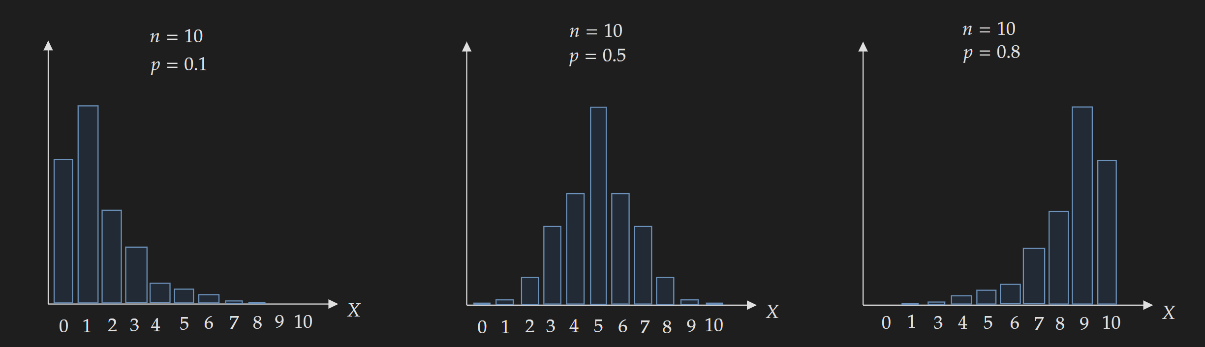
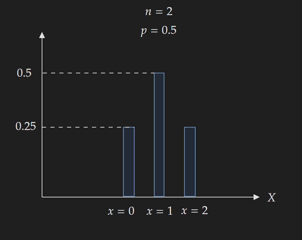 The shape of the PMF is determined by the value of $n$ and $p$
Changing the value of $n$ and $p$ change the shape of the distribution:
As a general thumb rule, we can say the following:
- $p=0.5$: Distribution will be symmetrical
- $p<0.5$: Distribution skewed to the left
- $p>0.5$: Distribution skewed to the right
⯌ Expected Value:
\[\boxed{E(x)=np}\]⯌ Variance:
\[\boxed{Var(x)=np(1-p)}\]⯌ Properties and Key Facts:
- Involves $n$ independent Bernoulli trials
- Applicable when a repeating process can result in two possible outcomes.
- The number of trials is fixed to $n$ and the number of successes is the random variable $x$
⯌ External Resources:
A nice visual introduction to beginners: From Primer
- How the probability shape changes with parameter change: From Simply Learning Pro
- A more deeper dive: From 3Blue1Brown
⯈ Multinomial Distribution
Let’s start with modifying the binomial distribution and write it in a different way:
- Assume $p_{1}$ is the probability of outcome 1 and $p_{2}$ is the probability of outcome 2.
- Also, assume that, out of $n$ trials $x_{1}$ times the outcome 1 happens and $x_{2}$ times the outcome 2 happens.
- As these outcomes are mutually exclusive $n=x_{1}+x_{2}$
Then the binomial distribution can be written in the following form:
\[P(X_{1}=x_{1}, X_{2}=x_{2}|p_1, p_2)= \frac{n!}{x_{1}!~x_{2}!}~ p^{x_{1}}_{1}~ p_{2}^{x_{2}}\]Now we can extend it to $K$ different category rather than thinking about $2$ category. For $K$ different possibilities with $p_k$ and $x_k$ being the probability and count for the $k$ th category, $k=1,…,K$.
\[P(X_{1}=x_{1}, X_{2}=x_{2}, \cdots,X_{K}=x_{K}|p_1, p_2, \cdots, p_{K})= \frac{n!}{x_{1}!~x_{2}! \cdots x_K!}~ p^{x_{1}}_{1}~ p_{2}^{x_{2}} \cdots p^{x_{K}}_{K}\]We can express it more formally as follows:
\[\boxed{P(X_{1}=x_{1}, X_{2}=x_{2}, \cdots,X_{K}=x_{K}|p_1, p_2, \cdots, p_{K})= \frac{n!}{\prod_{k=1}^{K}x_{k}!}~ \prod_{k=1}^{K} p^{x_{k}}_{k}}\]where,
- $n=x_1+x_2+\cdots+x_{K}$
- $p_1+p_2+\cdots+p_K=1$
Also, another way I have seen this expressed in literature is as follows:
\[\binom{n}{x_1\ldots x_K} \prod_{k=1}^{K} p^{x_{k}}_{k}\]⯌ Properties and Key Facts:
- $p_1,p_{2},\cdots, p_{K}$ remains same from trial to trial
- It is a generalization of binomial distribution for $K$ number of probabilities
⯈ Multinoulli/Categorical Distribution
This distribution often gets mixed up with other distributions (specifically multinomial distribution) in the literature.
This can be thought of as a generalization of the Bernoulli distribution of K-states. For the Bernoulli distribution, I think of a biased coin, for the Multinouli distribution I think of a K-sided die. This means each K-state has some probability associated with it. As an example, for a fair 6-sided die, the probability for each side is $1/6$. The random variable is $X={x_1,x_2,\ldots,x_K}$. But it is better to think of it as a vector where one of the values can be $1$ while the others remain equal to $0$. For example if $K=3$, the possible states for the vector are:
\[[1,0,0] \\ [0,1,0] \\ [0,0,1]\]If you know about one-hot encoding this will seem familiar to you.
⯌ Probability Density Function:
\[\prod_{k=1}^{K} p^{x_{k}}_{k}\]This means we are multiplying the probability of each K-side coming up.
⯌ Property and Key Facts:
- This distribution is a special case of the multinomial distribution when number of trials $n=1$.
⯈ Geometric Distribution
⯌ Probability Density Function:
\[\boxed{P(X=x \mid p)= (1-p)^{x-1}~p}\]where,
- $p$ is the probability of success for an individual Bernoulli trial
- $(1-p)$ is the probability of failure for an individual Bernoulli trial
- $x$ is the random variable where $x$ is the trial number when first success happens
- $x-1$ trials results in failure, $x^{th}$ trial results in success
⯌ Cumulative Density Function:
\[\boxed{\operatorname{P}(X\leq x )=1- (1-p)^{x}}\]⯌ Expected Value:
\[\boxed{E(X)=\frac{1}{p}}\]⯌ Variance:
\[\boxed{Var(X)=\frac{1-p}{p^2}}\]⦿ Continuous Probability Distributions
⯈ Gaussian Distribution
⯌ Probability Density Function:
\[\boxed{f(x \mid \mu, \sigma)= \frac{1}{\sqrt{2\pi \sigma^{2}}} \exp\left({-\frac{(x-\mu)^{2}}{2\sigma^{2}}}\right)}\]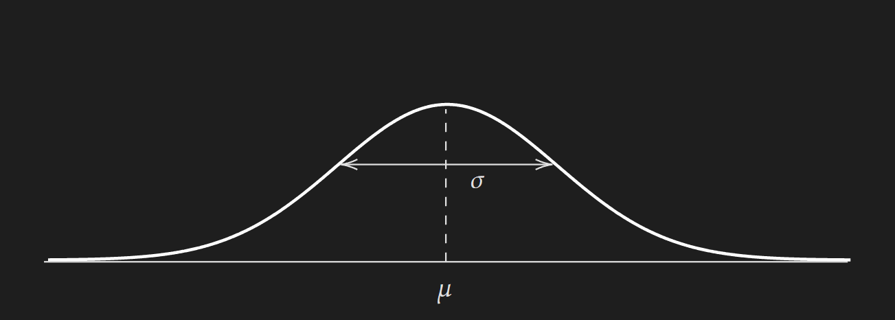
⯌ Cumulative Density Function:
No Closed-Form Analytical Equation
⯌ Expected Value:
\[\boxed{E(x)=\mu}\]⯌ Variance:
\[\boxed{Var(x)=\sigma^{2}}\]⯌ Multivariate case (PDF):
\[f(x \mid\mu, \Sigma)=\frac{1}{(2 \pi)^{D / 2}|\Sigma|^{1 / 2}} \exp \left\{-\frac{1}{2}(\mathbf{x}-\mu)^{\top} \Sigma^{-1}(\mathbf{x}-\mathbf{\mu})\right\}\] \[\text{where}, \mu \in \mathbb{R}^{D}, \Sigma \in \mathbb{R}^{D \times D}~\text{and}~\Sigma \succ0\]Here,
- $D$ is the number of dimensions
- $\mu$ is the mean vector
- $\Sigma$ is the covariance matrix
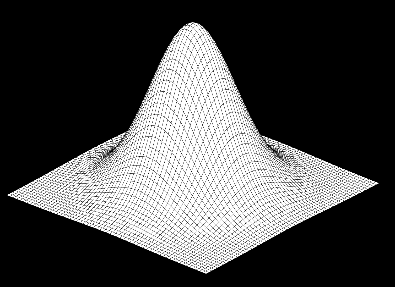 Bivariate Guassian PDF
To get a better appreciation of the formula we can consider the bivariate case where the number of dimensions $D=2$. For $D=2$,
\[x=\begin{bmatrix} x_1 \\ x_2\end{bmatrix} \qquad \mu=\begin{bmatrix} \mu_1 \\ \mu_2 \end{bmatrix} \qquad \Sigma=\begin{bmatrix} \sigma^{2}_{1} & \sigma_{12} \\ \sigma_{21} & \sigma_{2}^{2}\end{bmatrix}\]With these considerations, the bivariate Gaussian pdf can be expressed as follows:
\[f(x \mid\mu, \Sigma) = \frac{1}{(2\pi)^{2/2}\begin{vmatrix} \sigma^{2}_{1} & \sigma_{12} \\ \sigma_{21} & \sigma_{2}^{2}\end{vmatrix}^{1/2} } \exp \left(-\frac{1}{2}\begin{bmatrix} x_1 \\ x_2\end{bmatrix}^{\top} \begin{bmatrix} \sigma^{2}_{1} & \sigma_{12} \\ \sigma_{21} & \sigma_{2}^{2}\end{bmatrix}^{-1} \begin{bmatrix} x_1 \\ x_2\end{bmatrix} \right)\]To understand the nature of $\Sigma$ we can consider some special cases. First, let’s consider the off-diagonal elements $\sigma_{ij}=0$.
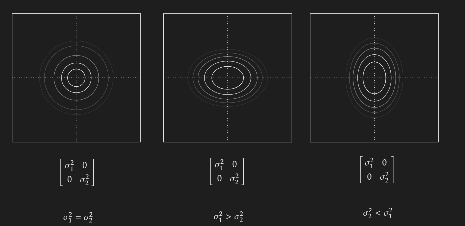
When the variance for both $x_{1}$ and $x_{2}$ are equal the contour plot is circular in nature. But when they are not equal the contour plot is elliptical in nature.
Now we can consider the case when the off-diagonal elements are not zero. One thing to note here as the covariance matrix is a symmetric matrix, $\sigma_{12}=\sigma_{21}$.
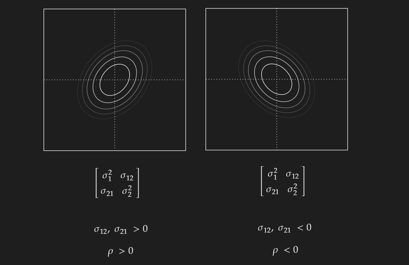
Depending on if they are positive or negative, it will be skewed towards a specific direction.
⯌ Marginalization of a multivariate Gaussian:
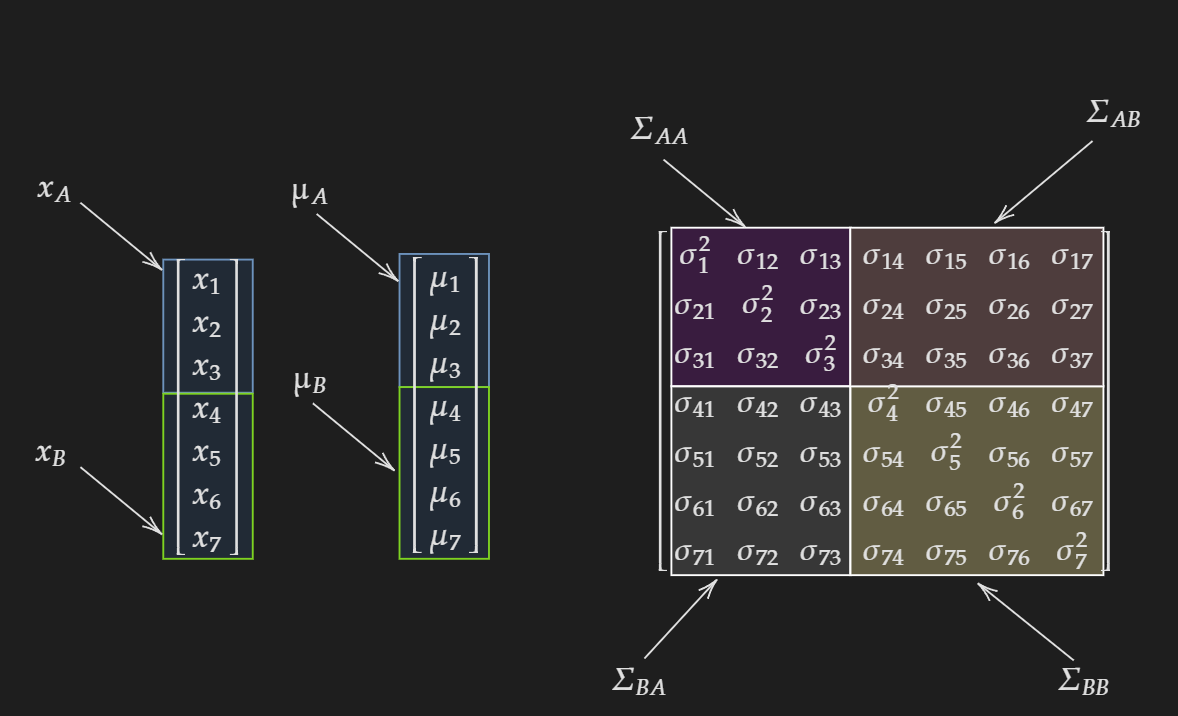
First, let us partition the random variable vector and the mean vector into two sections $A$ and $B$.
\[x= \begin{bmatrix} x_{1} \\ x_{2} \\ x_{3} \\ \vdots \\ x_{D-1} \\ x_{D}\end{bmatrix} = \begin{bmatrix} x_{A} \\ x_{B}\end{bmatrix}\] \[\mu= \begin{bmatrix} \mu_{1} \\ \mu_{2} \\ \mu_{3} \\ \vdots \\ \mu_{D-1} \\ \mu_{D}\end{bmatrix} = \begin{bmatrix} \mu_{A} \\ \mu_{B}\end{bmatrix}\]For the covariance matrix this will result in partitioning the matrix into four sections:
\[\Sigma= \begin{bmatrix} \Sigma_{AA} & \Sigma_{AB} \\ \Sigma_{BA} & \Sigma_{BB} \end{bmatrix}\]For me personally, the first time I saw this I did not get it. Because nobody showed me a visualization for a specific case. So, the visualization for $D=7$ and partitioned into $3$ and $4$ is shown below:
Back to the general case. Now let’s say we want to find the multivariate joint distribution of $x_{A}$. This means we need to integrate out all variables $x_{B}$.
Therefore the marginal of $x_{A}$ will be:
\[\boxed{x_{A} \sim \mathcal{N}(\mu_{A}, \Sigma_{AA})}\]Similarly, if we want to find the multivariate joint distribution of $x_{B}$. This means we need to integrate out all the variables $x_{A}$.
Therefore the marginal of $x_{B}$ will be:
\[\boxed{x_{B} \sim \mathcal{N}(\mu_{B},\Sigma_{BB})}\]This means if we know $\mu$ and $\Sigma$, in order to find $x_{A}$ and $x_{B}$ we can directly read off from $\mu$ and $\Sigma$ to construct the corresponding mean vector and covariance matrix.
\[\boxed{\text{Gaussian Distribution is closed under marginalization}}\]⯌ Conditioning on a multivariate Gaussian:
Conditioning on a multivariate Gaussian can be done with the following equations:
\[x_A \mid x_B \sim N\left(\mu_A+\Sigma_{A B} \Sigma_{B B}^{-1}\left(x_B-\mu_B\right), \Lambda_{A A}\right)\] \[x_B \mid x_A \sim N\left(\mu_B+\Sigma_{B A} \Sigma_{A A}^{-1}\left(x_A-\mu_A\right), \Lambda_{B B}\right)\] \[\text { where } \Lambda_{B B}=\Sigma_{B B}-\Sigma_{B A} \Sigma_{A A}^{-1} \Sigma_{A B}\] \[\text { where } \Lambda_{A A}=\Sigma_{A A^{-}} \Sigma_{A B} \Sigma_{B B}{ }^{-1} \Sigma_{B A}\]I am not gonna show the proof because it is way too rigorous and knowing it gives too little intuition for me to cover in this article.
\[\boxed{\text{Gaussian Distribution is closed under conditioning}}\]⯌ Affine transformation:
If we consider a multivariate gaussian distribution $x\sim \mathcal{N}(\mu,\Sigma)$ then performing an affine transformation to $x$ to get another random variable $z$ can be done as follows:
\[z = Ax+b\] \[\text{where,} ~A \in \mathbb{R}^{D\times D}~\text{and}~b\in \mathbb{R}^{D}\]Then the random variable $z$ will also follow a Gaussian distribution as follows:
\[z \sim \mathcal{N}(A \mu+b,A \Sigma A^{\top})\] \[\boxed{\text{Gaussian Distribution is closed under affine transformation}}\]⯈ Student-t Distribution
At first glance, this looks really complicated and the way to get around it is not to look at the constant part and only focus on the kernel part. Personally, I only had to deal with the explicit version of the student-t distribution when doing Bayesian stuff. When using it in other scenarios like dealing with sampling distribution, you almost never have to deal with the explicit version of the PDF, it’s taken care of by the software package you are using.
⯌ Probability Density Function:
\[f(t \mid v)=\frac{\Gamma\left(\frac{v+1}{2}\right)}{\Gamma\left(\frac{v}{2}\right)} \frac{1}{\sqrt{v \pi}} \frac{1}{\left(1+\frac{1}{v} t^2\right)^{(v+1) / 2}}\]where,
- $v$ is the degrees of freedom
- $\Gamma$ is the gamma function defined as $\Gamma(n)=(n-1)!$
⯌ Expected Value:
\[E(x)=\begin{cases} \mu ,~ \text{when} ~ v>1\\ \\ \text{undefined}, ~ \text{otherwise} \end{cases}\]⯌ Variance:
\[Var(X)=\begin{cases} \frac{v}{v-2}, v>2 \\ \\ \infty, 1 <v \leq2 \\ \\ \text{undefined},~\text{otherwise} \end{cases}\]⯌ Multivariate Case:
\[f(s \mid v, \delta, \mathrm{T})=\frac{\Gamma\left(\frac{v+p}{2}\right)|\mathrm{T}|^{-1 / 2}}{(v \pi)^{p / 2} \Gamma\left(\frac{v}{2}\right)} \frac{1}{\left[1+\frac{1}{v}(s-\delta)^{\prime} \mathrm{T}^{-1}(s-\delta)\right]^{(v+p) / 2}}\]where,
- $p$ is the number of dimensions
- $v$ is the degrees of freedom
- $\delta$ is the location parameter
- $T$ is the scale matrix
where,
\[\frac{v}{v-2} \mathrm{~T}=\Sigma\]The expectation is given by:
\[\boxed{E(S \mid \nu, \delta, \mathrm{T})=\delta}\]The covariance is given by:
\[\operatorname{cov}(S \mid \delta, \mathrm{T})=\frac{v}{v-2} \mathrm{~T}=\Sigma\]⯌ Properties and Key Facts:
The larger the value of degrees of freedom $v$, the more it gets closer to the normal distribution. You will find a nice interactive visualization here to understand how it approaches a normal distribution as the degrees of freedom increase.
Whenever you have to deal with samples there is a very high chance you will need to deal with the student-t distribution in some way.
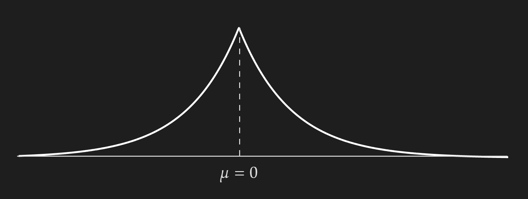
⯈ Laplace/Double-Sideded Exponential Distribution
⯌ Probability Density Function:
\[f(x \mid \mu, b)=\frac{1}{2 b} \exp \left(-\frac{|x-\mu|}{b}\right)\] \[\text{where}, b>0\]where,
- $\mu$ is the location parameter
- $b$ is the scale parameter
⯌ Cumulative Density Function:
\[\operatorname{F_{X}}(X\leq x )= \begin{cases} \frac{1}{2} \exp \left(\frac{x-\mu}{b}\right) & \text { if } x \leq \mu \\ \\ 1-\frac{1}{2} \exp \left(-\frac{x-\mu}{b}\right) & \text { if } x \geq \mu \end{cases}\]⯌ Expected Value:
\[\boxed{E(X)=\frac{1}{p}}\]⯌ Variance:
\[\boxed{Var(X)=2b^2}\]⯈ Beta Distribution
Beta distribution is completely parameterized by $\alpha$ and $\beta$. Normally the $\alpha$ is called the “successful outcomes” and $\beta$ is called “unsuccessful outcomes”. Please note that we use the terms “successful” and “unsuccessful” as placeholder. A better way to think is an event that has two possible outcomes, where one outcome is termed as the “success” and the other outcome is termed as “unsuccessful”.
External Resources:
- To get a more intuitive feeling about the Beta distribution I would recommend looking at this video from Luis Serrano.
⯌ Probability Density Function:
\[\boxed{f(x \mid \alpha, \beta)=\frac{\Gamma(\alpha+\beta)}{\Gamma(\alpha) \Gamma(\beta)} x^{\alpha-1}(1-x)^{\beta-1}}\] \[\text { where, } \alpha, \beta>0, x \in[a, b]\]Here, $\Gamma(x)$ is the gamma function defined as $\Gamma(x-1)!$
Also, $\frac{\Gamma(\alpha+\beta)}{\Gamma(\alpha) \Gamma(\beta)}$ is sometimes expressed as $\frac{1}{B(\alpha_1,\alpha_2)}$ which is the normalizing factor.
⯌ Cumulative Density Function:
No Closed-Form Analytical Equation
⯌ Expected Value:
\[\boxed{E(x)=\frac{\alpha}{\alpha+\beta}}\]⯌ Variance:
\[\boxed{Var(x)=\frac{\alpha \beta}{(\alpha+\beta)^2(\alpha+\beta+1)}}\]⯌ Special case for uniform distribution:
if $\alpha=1$ and $\beta=1$ then, the beta distribution represents a uniform distribution.
⯌ Properties and Key Facts:
- Known as “The Probability Distribution of Probabilities”.
- Bounded between $0$ to $1$. As it signifies the distribution of probability values it does not make sense for it to have a value not within the range $0$ to $1$.
- Suitable distribution model for the random behavior of percentages and proportions.
- Has a close connection to binomial distribution. Beta is the conjugate prior to Binomial distribution.
⯈ Gamma Distribution
⯌ Probability Density Function:
\[\boxed{f(x \mid \alpha, \beta)=\frac{\beta^\alpha}{\Gamma(\alpha)} x^{\alpha-1} \mathrm{e}^{-\beta x}}\]There is another version of this distribution with only one parameter $\alpha$.
⯌ Cumulative Density Function:
No Closed-Form Analytical Equation
⯌ Expected Value:
\[\boxed{E(x)=\alpha / \beta}\]⯌ Variance:
\[\boxed{Var(x)=\alpha / \beta^{2}}\]⯈ Inverse Gamma Distribution
⯌ Probability Density Function:
\[\boxed{f(x \mid \alpha, \beta)=\frac{\beta^\alpha}{\Gamma(\alpha)} x^{-\alpha-1} \mathrm{e}^{-\beta / x}}\] \[\text { where, } \alpha, \beta>0,0<x<\infty\]⯌ Cumulative Density Function:
No Closed-Form Analytical Equation
⯌ Expected Value:
\[\boxed{E(x)=\frac{\beta}{\alpha-1}}\]⯌ Variance:
\[\boxed{Var(x)=\frac{\beta^2}{(\alpha-1)^2(\alpha-2)}}\]⯈ Dirichlet distribution
To really understand Dirichlet distribution you first need to understand the Beta distribution because Dirichlet distribution is the generalization of the Beta distribution. The other way to think about this is the Beta distribution is the special case of the Dirichlet distribution when $K=2$.
⯌ Probability Density Function:
\[f(x_1,x_2,\cdots, x_K \mid \alpha_1, \alpha_2, \cdots, \alpha_K)=\frac{1}{B(\alpha)} \prod_{k=1}^{K}x_{k}^{\alpha_k -1}\] \[\text { where, } B(\alpha)= \frac{\prod_{k=1}^{K} \Gamma(\alpha_{k})}{\Gamma(\sum_{k=1}^{K}\alpha_{k})}, \text{which is the normalization factor}\]Properties and Key Facts:
- The input to the distribution is a vector and what we sample from the distribution is also a vector.
- It is a multivariate generalization of the beta distribution.
- Dirichlet is the conjugate prior of the categorical and multinomial distribution.
⯈ $\chi^{2}$ Distribution:
If $Z_1, \ldots, Z_\nu$ are independent, standard normal random variables, then the sum of their squares, \(Q=\sum_{i=1}^k Z_i^2,\) is distributed according to the chi-squared distribution with $\nu$ degrees of freedom. This is usually denoted as
\[Q \sim \chi^2(\nu) \text { or } Q \sim \chi_{\nu}^2\]⯌ Probability Density Function:
\[f(x \mid \nu)=\frac{x^{\frac{\nu}{2}-1} e^{-\frac{x}{2}}}{2^{\nu / 2} \Gamma(\nu / 2)}\] \[\text{where,}~ x>0\]⯌ Expectation:
\[\nu\]⯌ Variance:
\[2 \nu\]⯌ Relationship to sampling variance:
Now, consider a random sample of size $n$ from a normal distribution with unknown variance $\sigma^2$ The sample variance $S^2$ is given by:
\[S^2=\frac{1}{n-1} \sum_{i=1}^n\left(X_i-\bar{X}\right)^2\]where $X_i$ are the individual sample observations, and $\bar{X}$ is the sample mean.
The sampling distribution of $S^2$ (scaled by $\sigma^2$ ) follows a chi-squared distribution with $n-1$ degrees of freedom: \(\frac{(n-1) S^2}{\sigma^2} \sim \chi^2(n-1)\)
Note that this is not the distribution of exact $S^2$, rather it is the distribution for $\frac{(n-1) S^2}{\sigma^2} $.
Properties and Key Facts:
- The multivariate generalization of the $\chi^2$ distribution is the Wishart distribution.