Prerequisites for Convex Optimization 2

This post is a continuation of my previous post Prerequisites for Convex Optimization 1. Here, I am going to cover more pre-requisite topics for understanding convex optimization. As I mentioned in the previous post, most of the topics are from Boyd.

Convex Combination

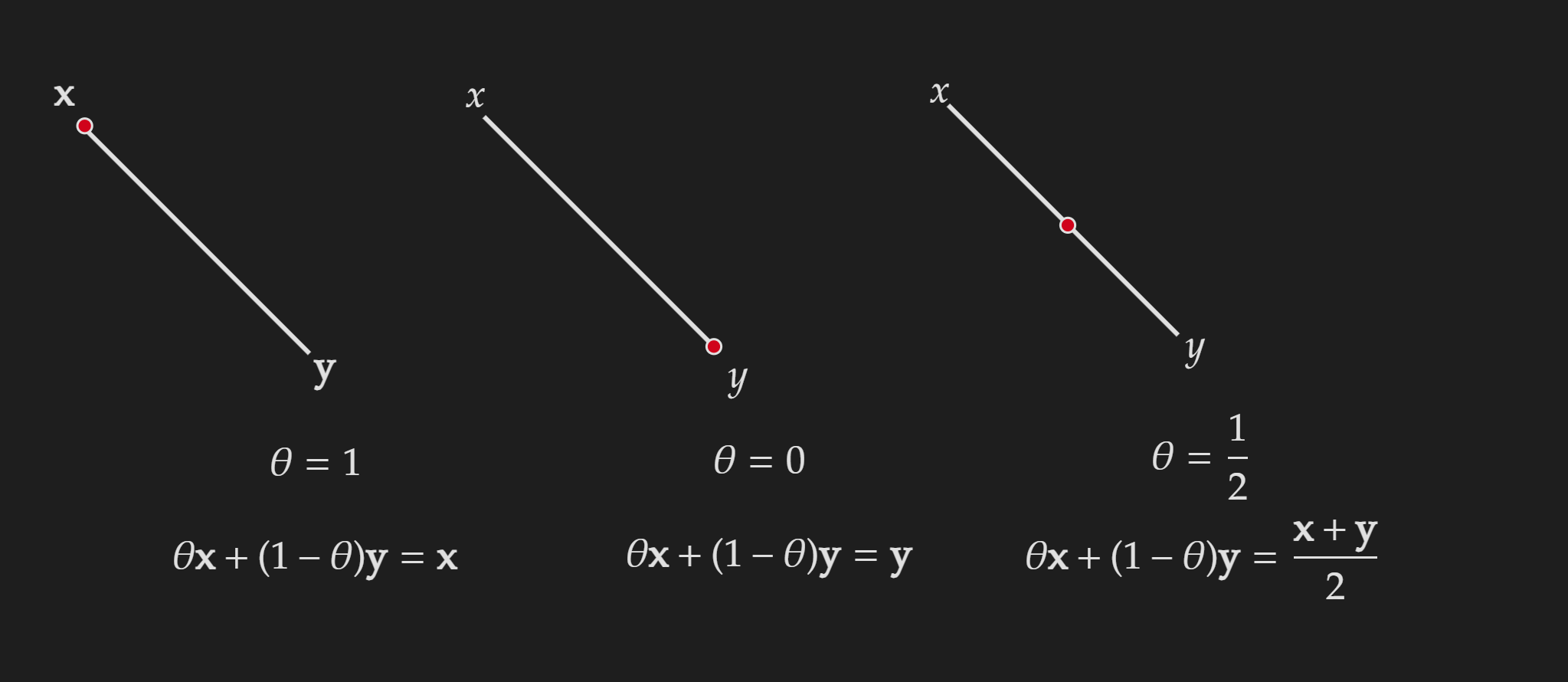
Let’s start with the convex combination of two points. This is pretty easy to understand because we used this concept to define a convex set and convex function.

Consider the following, which represents the convex combination of two points:

\[\theta \in[0,1] \quad \theta \mathbf{x}+(1-\theta) \mathbf{y}\]

A visualization is given below:

This gets tricky when we are dealing with more than two points. First, let’s take a look at the formal definition,

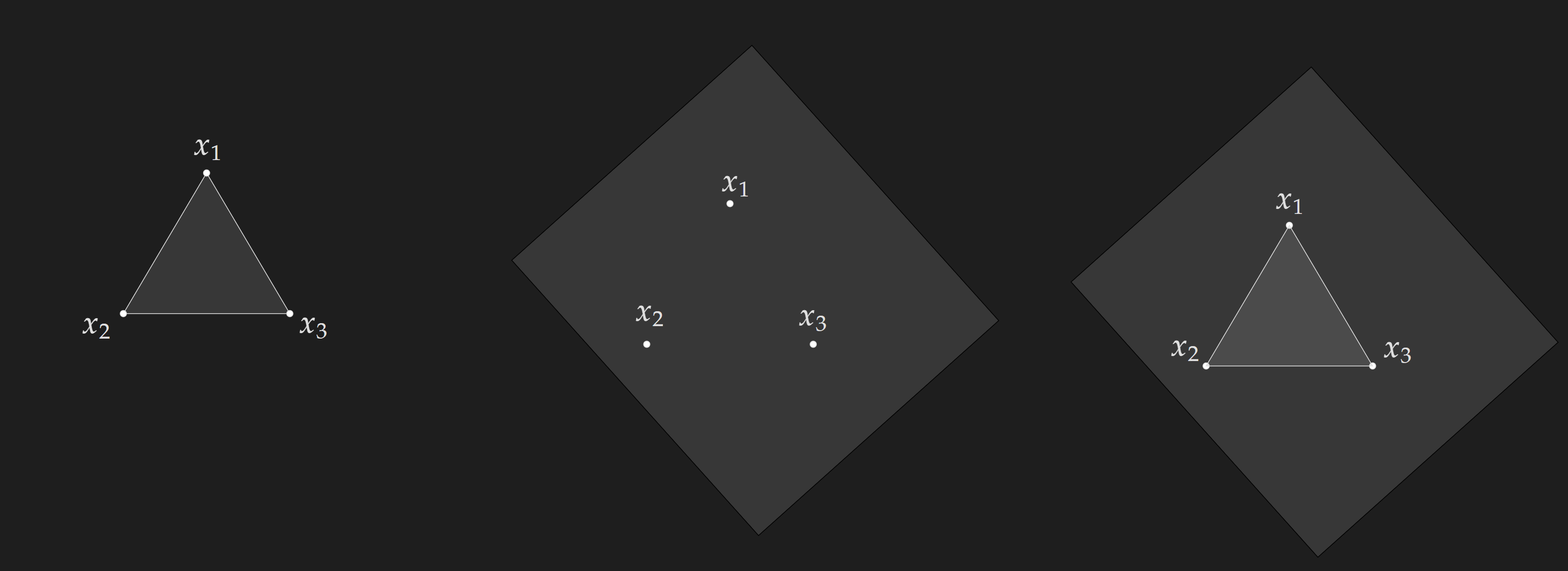
A convex combination of points $x_1,x_2,x_3,\cdots$ in a vector space is a linear combination of these points with non-negative coefficients that sum to $1$. Mathematically,

\[\theta_1 x_1+\theta_2 x_2+\ldots+\theta_k x_k\] \[\theta_i \geq 0\] \[\sum_{i=1}^k \theta_i=1\]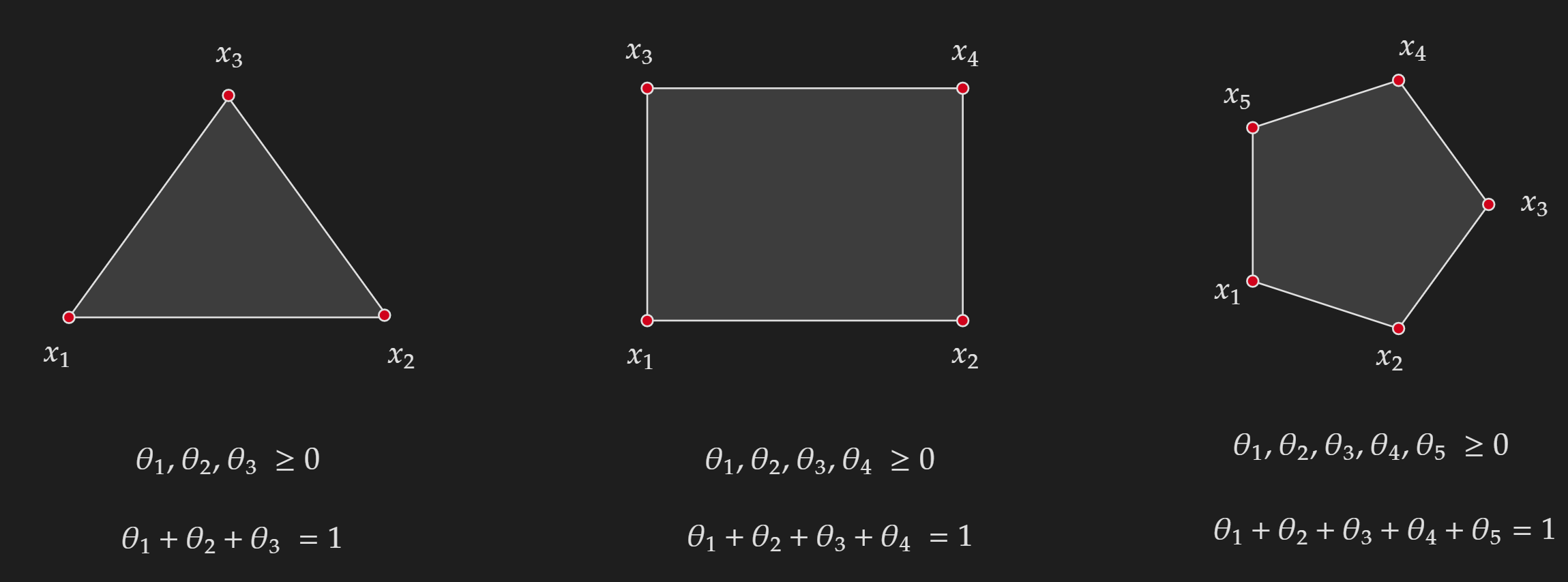

In my head, I visualize it as I am tuning knobs for $\theta_1,\theta_2,\theta_3, \cdots$ given a set of points $x_1,x_2,x_3\cdots$ and kind of filling in the area.

In a convex set, any convex combination of points in the set remains within the set.

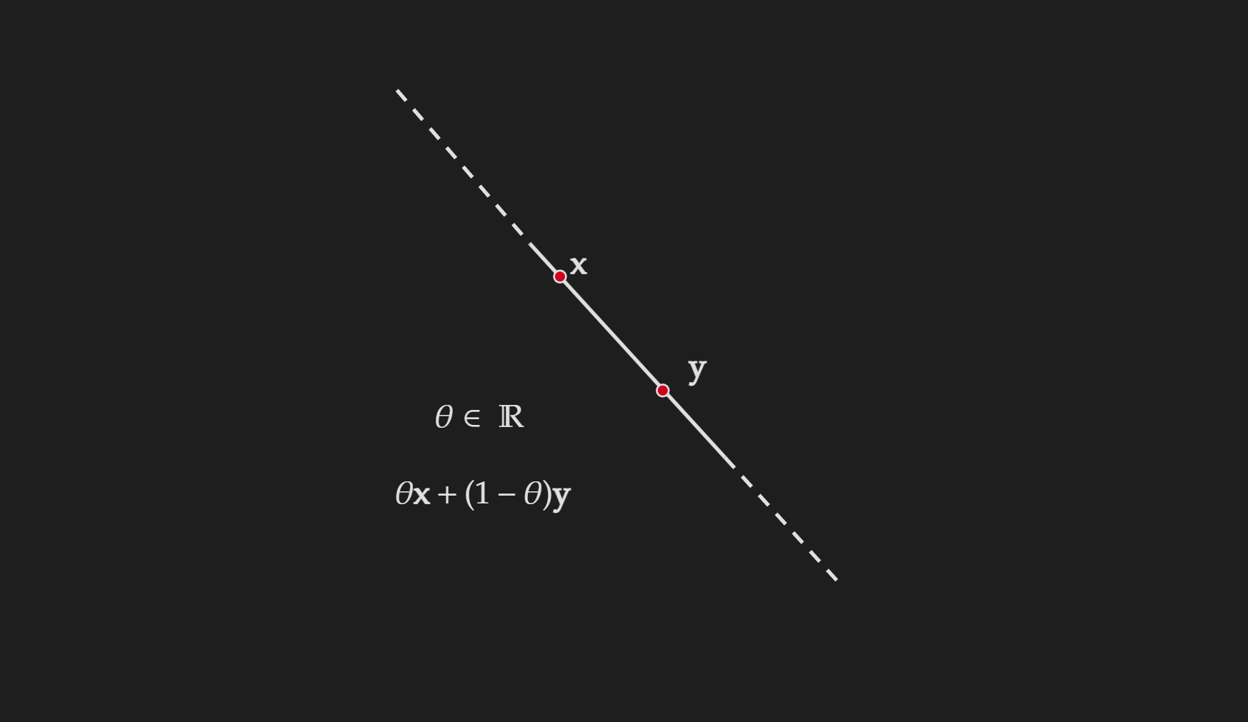
Affine Combination

\[\theta \mathbf{x}+(1-\theta) \mathbf{y}, \quad \theta \in \mathbb{R}\] \[\sum_{i=1}^k \theta_i=1\]

One important thing to notice here is the contrast with the convex combination. For the convex combination, we had another restriction for $\theta$.

Affine Set

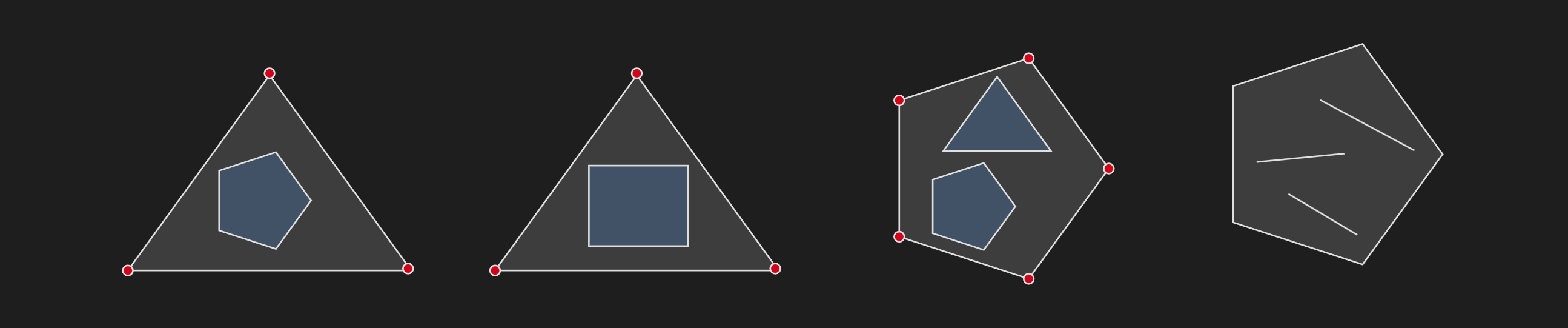
Contains the line through any two distinct points in the set. Think of it this way, you are given a set in $\mathbb{R}^n$, you pick two points from that set and draw a line that goes through those two points. Now all possible points on that line should be contained in that set. If that’s the case, then the set is affine.

One important thing to remember is every convex set is also affine, but not every affine set is convex. Convexity is a stronger condition than affineness. See the following visualization to get an intuitive understanding of it:

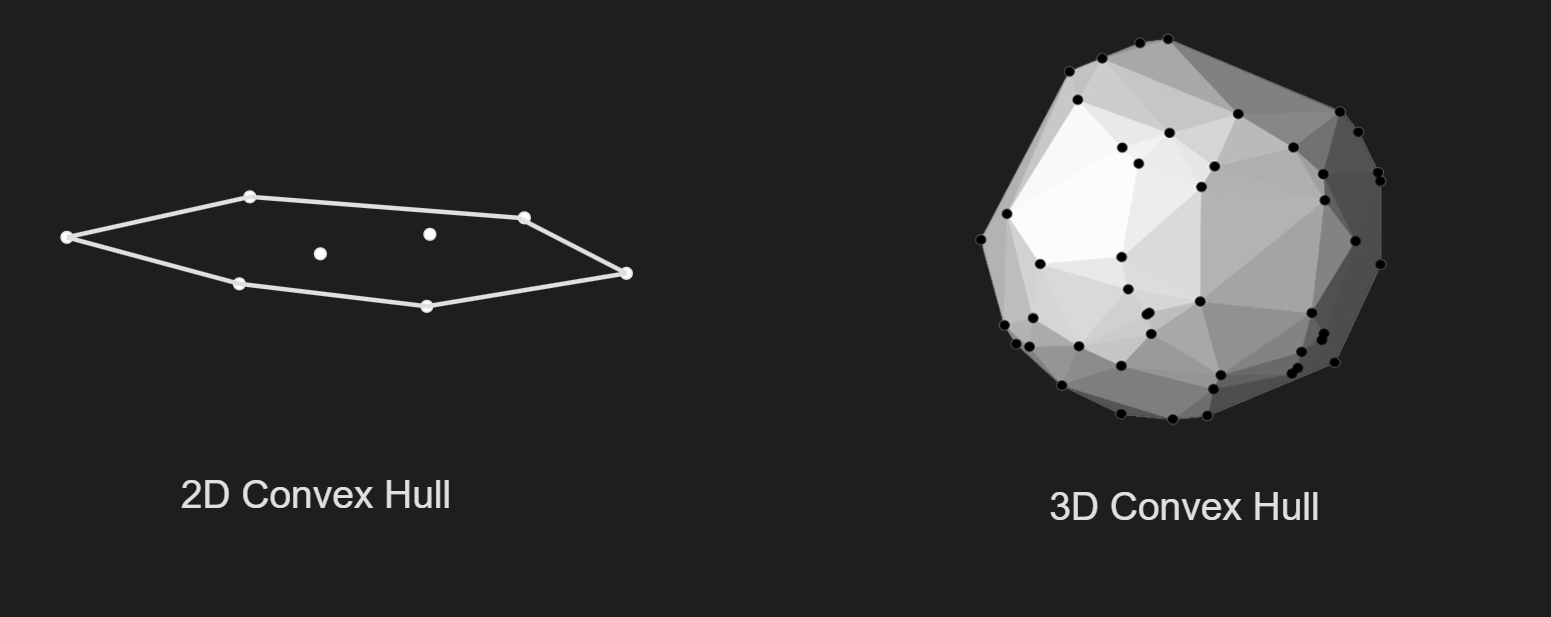
Affine Hull and Convex Hull

The definition of an affine hull:

\[\operatorname{aff}(S)=\left\{\sum_{i=1}^k \theta_i x_i \mid x_i \in S, \sum_{i=1}^k \theta_i=1, \theta_i \in \mathbb{R}\right\}\]

The definition of a convex hull:

\[\operatorname{conv}(S)=\left\{\sum_{i=1}^k \theta_i x_i \mid x_i \in S, \sum_{i=1}^k \theta_i=1, \theta_i \geq 0\right\}\]

These seem useless because they are kind of redefining the convex set and affine set. Well, convex hull and affine hull are themselves respectively convex and affine sets by definition. These become useful when you are given a set of points without structure and you want to form a convex set and affine set. The way you form those convex sets and affine sets is by creating the convex hull and affine hull from the set of given points. In addition, convex hull and affine hull have two special properties:

• The set $\mathbf{aff}(S)$ is the smallest affine set containing $S$.
• The set $\mathbf{conv}(S)$ is the smallest convex set containing $S$.

Conic Combination

The formal definition of conic combination for a set of points $x_1, x_2, \ldots, x_k$ is given below:

\[x_1, x_2, \ldots, x_k \in S\] \[\theta_1 x_1+\theta_2 x_2+\ldots+\theta_k x_k\] \[\theta_i \geq 0\]

Not that $\theta$ values do not need to add up to $1$, the only requirement they need to satisfy is, that they need to be greater or equal to $0$ (non-negative).

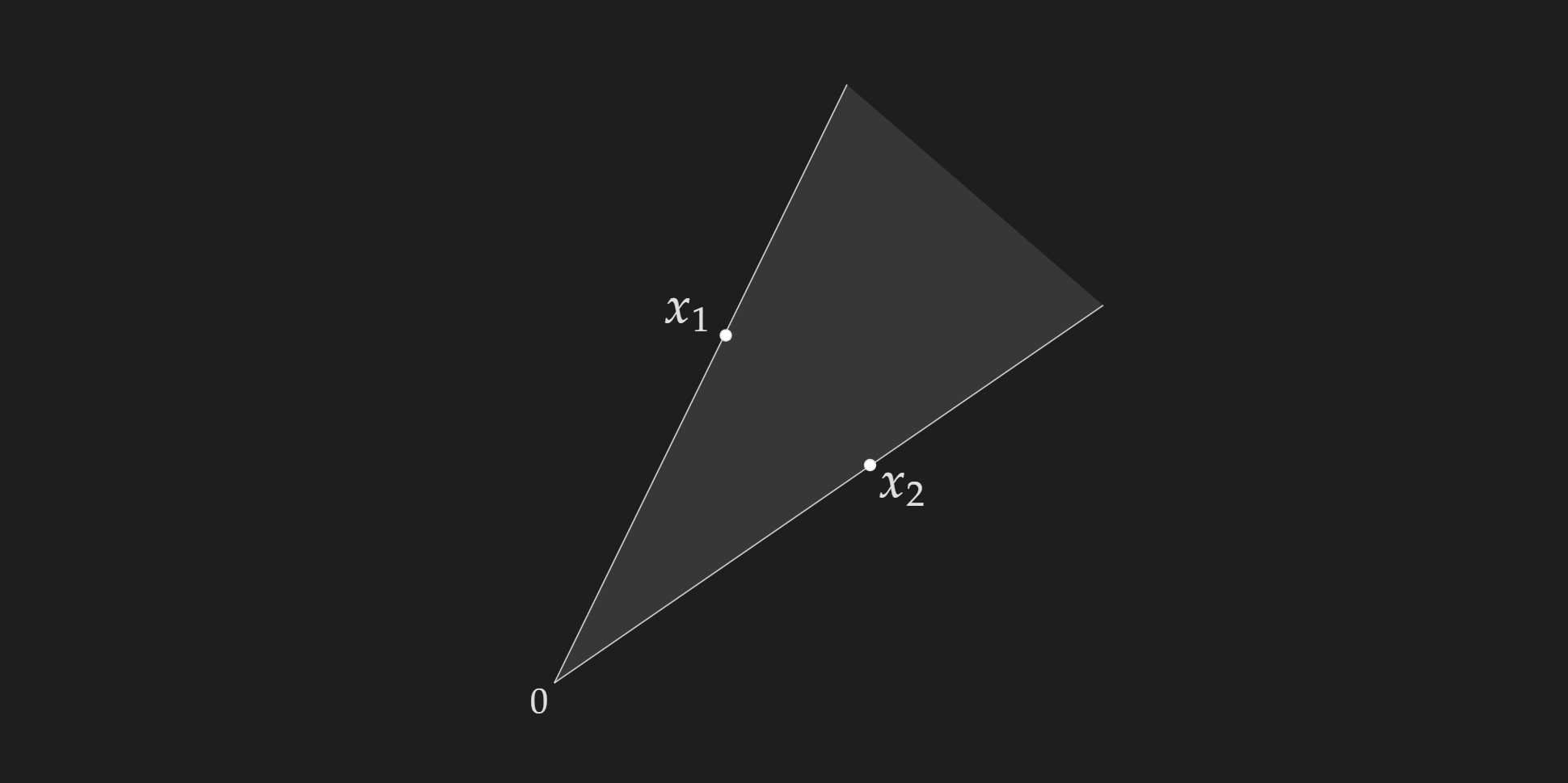
Convex Cone

The set $S$ is called a convex cone, if:

\[\forall x_1, x_2 \in S, \theta_1, \theta_2 \geq 0\] \[\theta_1 x_1+\theta_2 x_2 \in S\]

A visualization of a conic cone is given below:

Conic Hull

The conic hull can be formed with the following definition:-

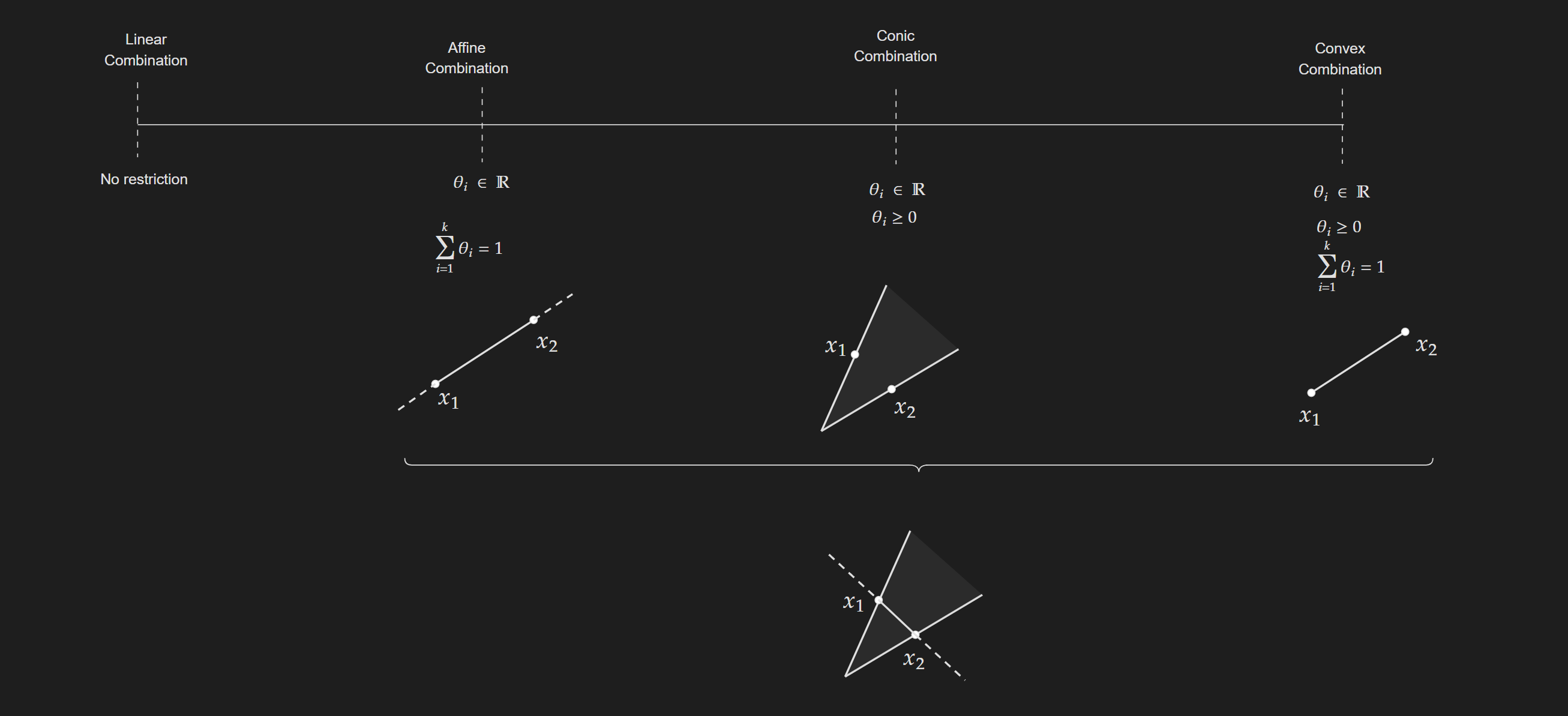
\[\operatorname{cone}(S)=\left\{\sum_{i=1}^k \theta_i x_i \mid x_i \in S, \theta_i \geq 0\right\}\]

Summarization of Convex, Affine and Conic Set

Keep the following figure in your head.

Hyperplanes

A hyperplane is a set which has the following form:

\[\left\{x \mid a^\top x=b\right\}(a \neq 0)\]

Note that, hyperplanes do not have the restriction of going through the origin (unlike vector subspaces). If you get confused imagine hyperplanes just are lines in $\mathbb{R}^2$ and surfaces in $\mathbb{R}^3$.

A couple of points about hyperplanes:

• A hyperplane separates $\mathbb{R}^n$ into two half-spaces.

• Hyplanes are both affine and convex.

A visualization of hyperplane:

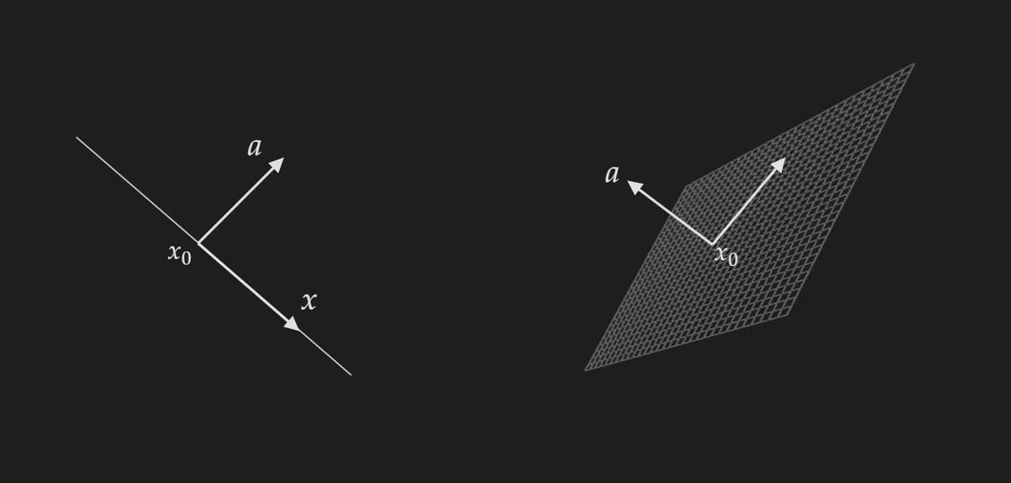
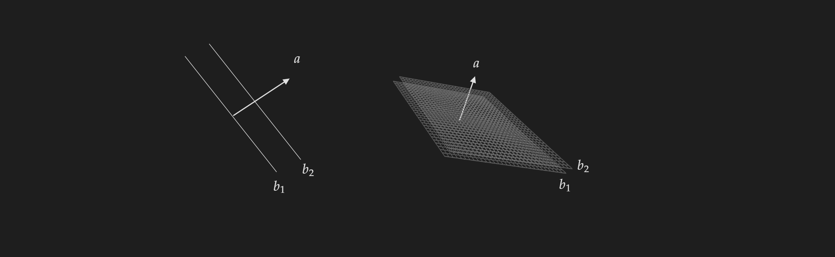
Now you need to have to visualization in your head:

• Tuning the vector $a$ kind of tilts the hyperplane. The direction of tilting kind of depends on which component of vector $a$ you are tuning.

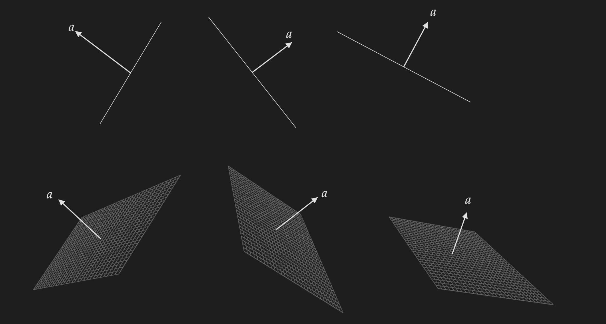
• Tuning the value $b$ kind of shifts the hyperplane without titling it (you need to keep vector $a$ fixed).

Half Spaces

A half-space is a set of points of the following form:

\[\left\{x \mid a^T x \leq b\right\}(a \neq 0)\]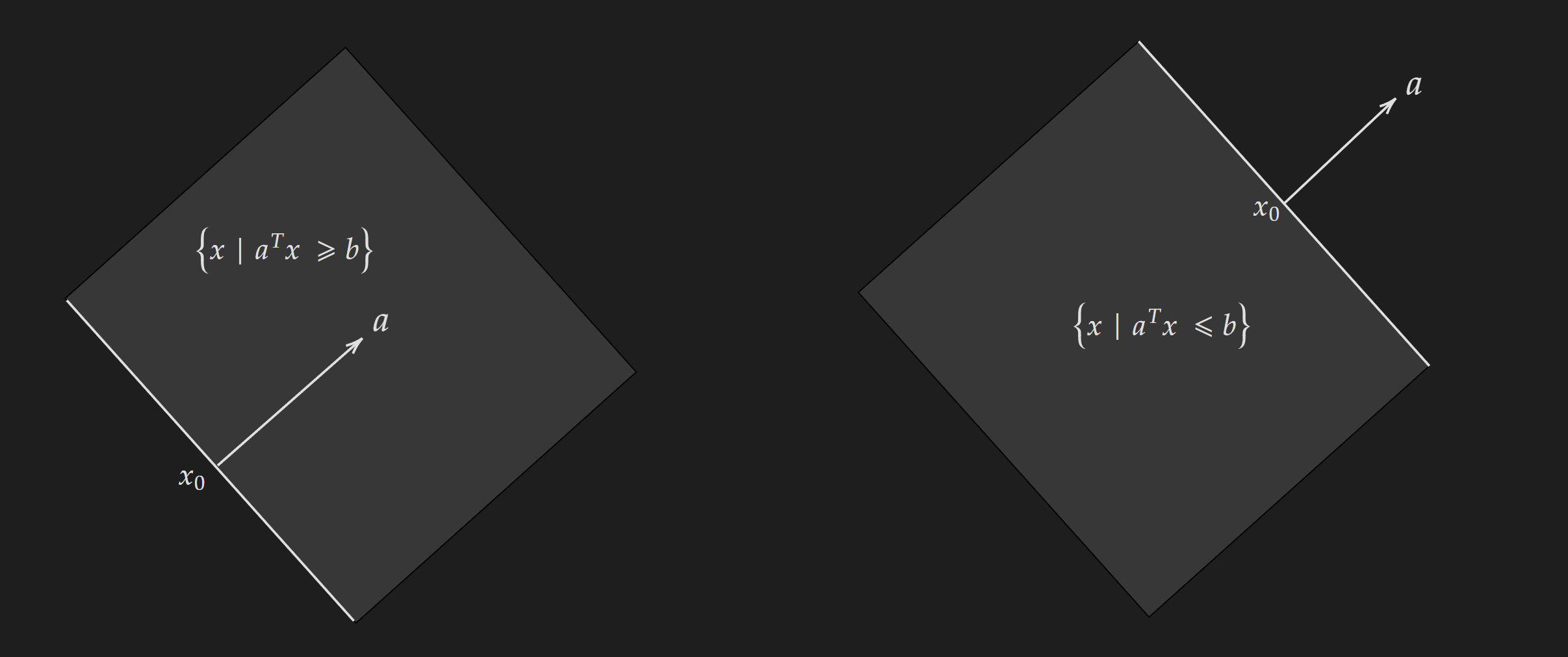

A couple of points about half-spaces:

• The equality part can be dropped, in that case, the half-space will not contain the points along the line.

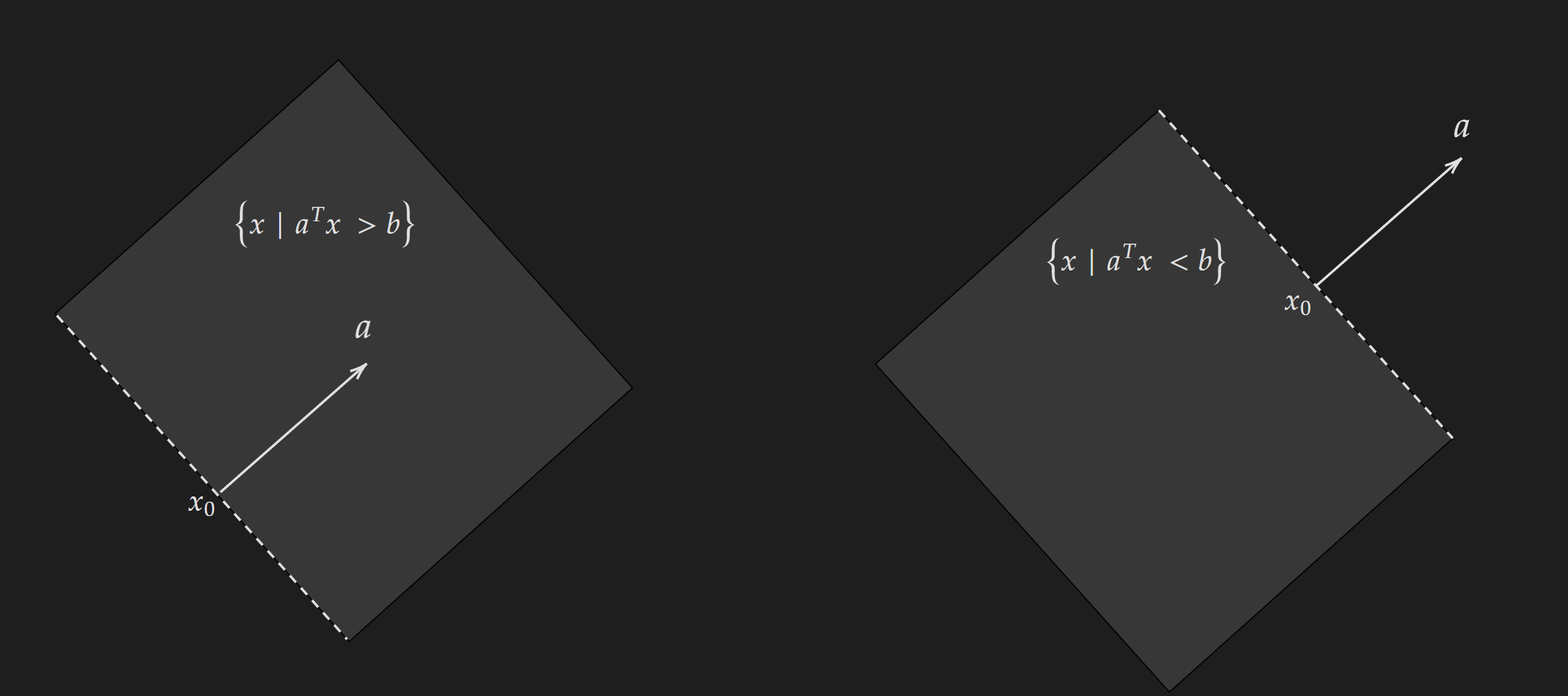
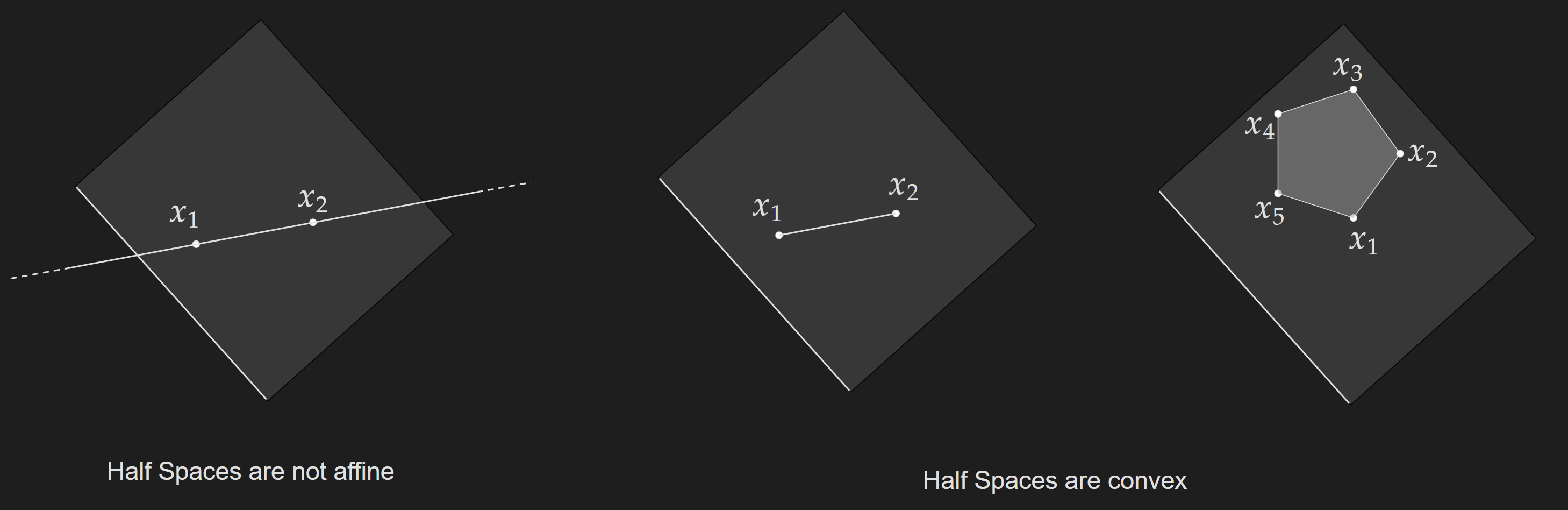
• A word of caution, even though it seems like half-spaces are just like vector spaces (or vector subspaces) they are not. That is if you pick two points (vectors) from the the half-space, a linear combination of them may fall outside the half-space. In other words, the points from the set are not closed under linear transformation.

• Half spaces are not affine set, they are convex set.

Euclidean Ball

A Euclidean ball is defined with two parameters $x_c$ which is the center of the ball and $r$ which is the radius of the ball.

\[B\left(x_c, r\right)=\left\{x \mid\left\|x-x_c\right\|_2 \leq r\right\}=\left\{x_c+r u \mid\|u\|_2 \leq 1\right\}\]

A visualization of the Euclidean ball is given below:

Ellipsoid

A generalization of the Euclidean ball can be done by incorporating a symmetric positive semidefinite matrix $P$.

\[\left\{x \mid\left(x-x_c\right)^T P^{-1}\left(x-x_c\right) \leq 1\right\}\] \[P \in \mathbf{S}_{++}^n\]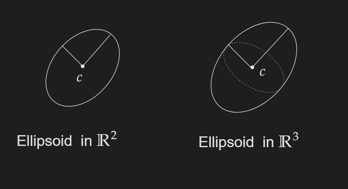

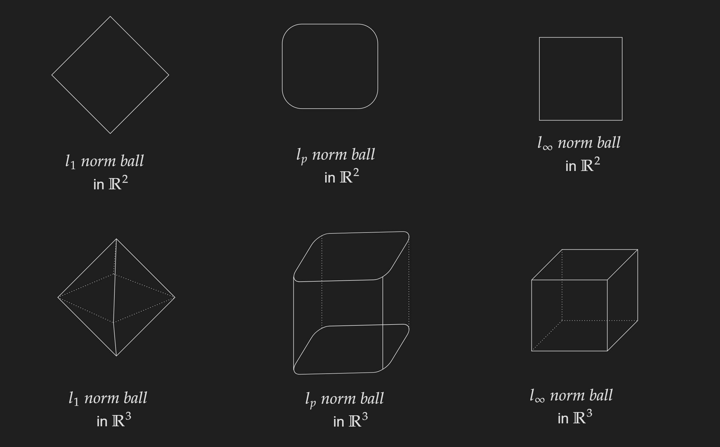
Norm Ball

A set of points defined by the following equation:

\[\left\{x \mid\left\|x-x_{\mathrm{c}}\right\| \leq r\right\}\]

This is generalized for any valid norm.

Norm Cone

The set of points which are defined as follows:

\[\{(x, t) \mid\|x\| \leq t\}\]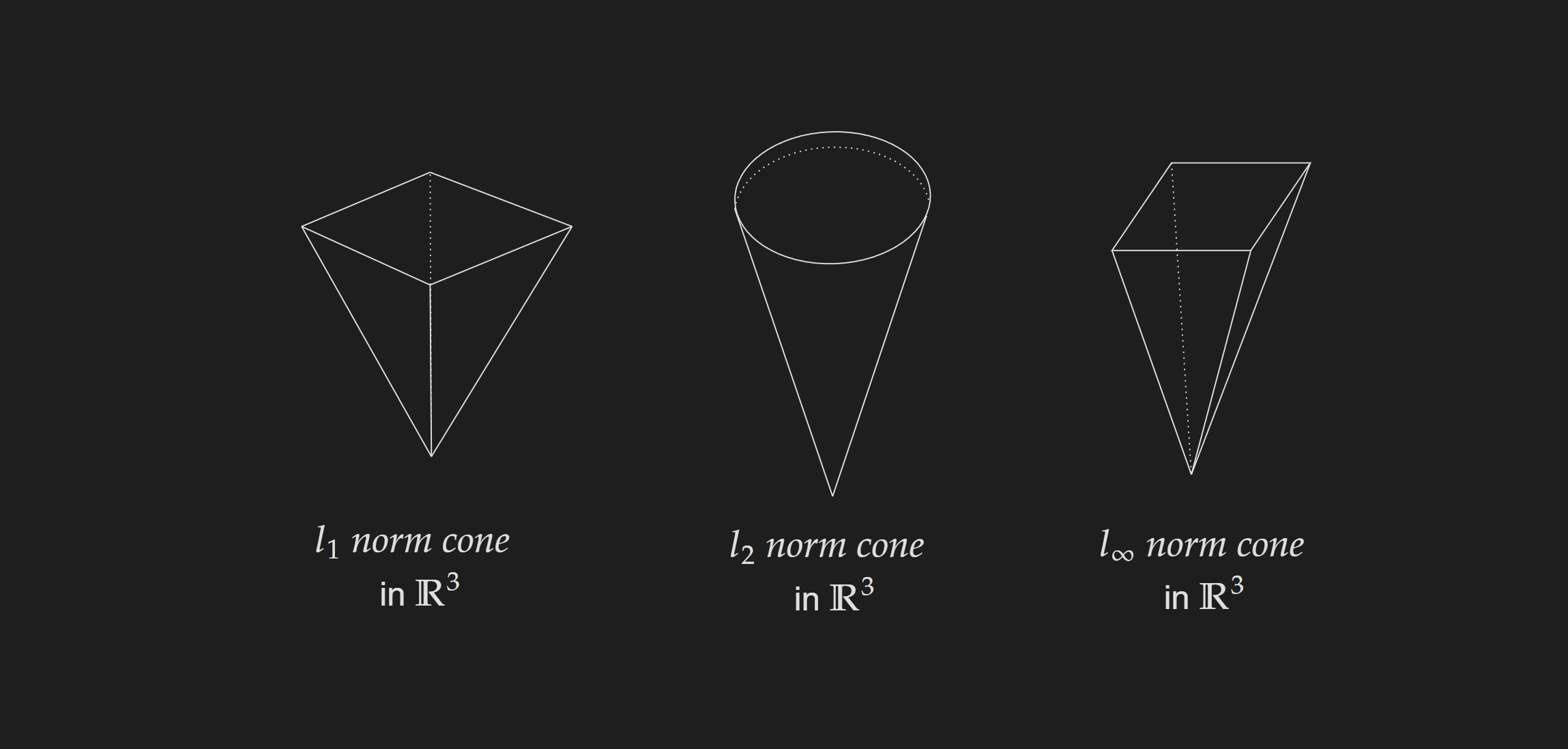

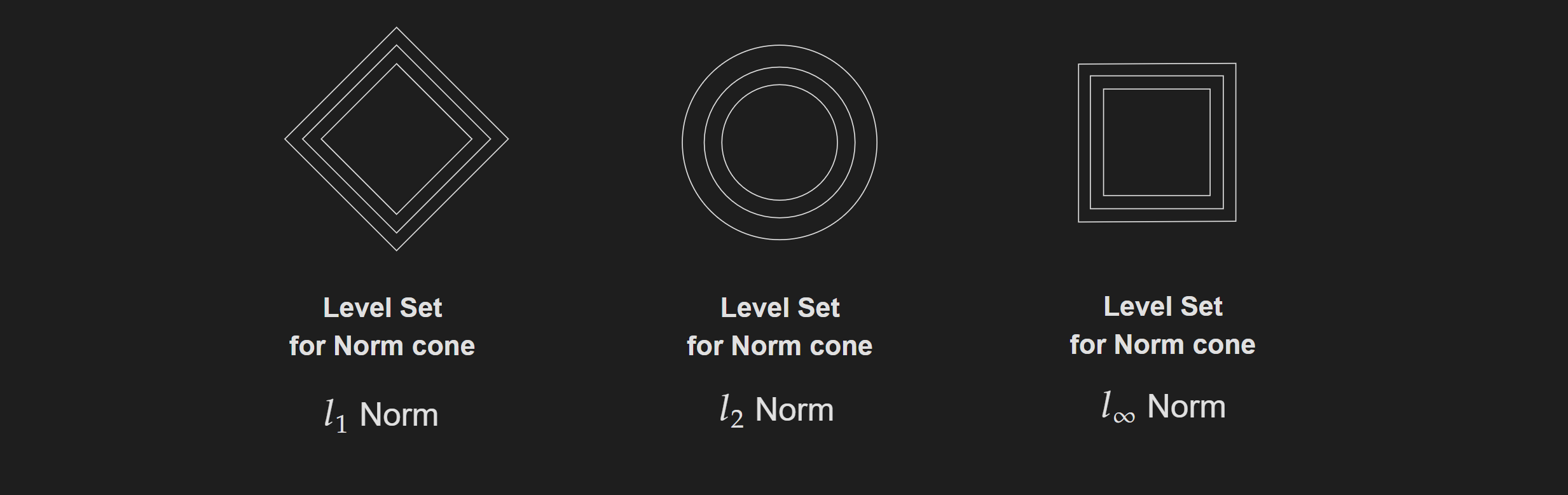
Visualize the level sets for these norm cones:

I will point to a Geogebra notebook by Peter J.C. Dickinson if you want to visualize these in 3D.

Polyhedra

A polyhedra is a set of points given by the following equation:

\[\left\{x \mid A x \preceq b, Cx=d \}\right.\] \[A \in \mathbf{R}^{\operatorname{mxn}}, C \in \mathbf{R}^{p \times n}, \preceq\text { is component wise inequality }\]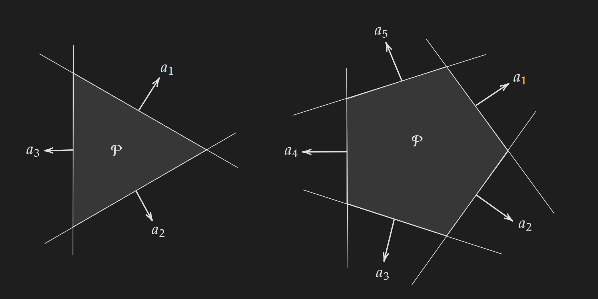

Polyhedra can also be thought of as:

• Intersection of finitely many half spaces and hyperplanes

• The solution set of many inequalities and equalities

Positive Semidefinite Cones

Before, we define this we need to get accustomed to some new notations.

Set Notation	Set Definition (1)	Set Definition (2)	Meaning
$\mathbf{S}^n$	———-	———-	Set of Symmetric $n \times n$ Matrices
$\mathbf{S}_{+}^n$	${X \in \mathbf{S}^n \mid X \succeq 0}$	$X \in \mathbf{S}_{+}^n \ \Longleftrightarrow z^T X z \geq 0$ for all $z$	Set of Positive Semi Definite $n \times n$ Matrices
$\mathbf{S}_{++}^n$	${X \in \mathbf{S}^n \mid X \succ 0 }$	$X \in \mathbf{S}_{++}^n \ \Longleftrightarrow z^T X z > 0$ for all $z$	Set of Positive Definite $n \times n$ Matrices

Now for $n \geq 3$, it is not possible to visualize the cone, so we will restrict ourselves to $n=2$.

Let’s consider a general symmetric matrix as follows:

\[X=\left[ \begin{aligned} x \qquad z \\ z \qquad y\end{aligned} \right]\]

Now if this matrix has to be positive semidefinite (meaning $X \in \mathbf{S}^{n=2}_{+}$) two things need to happen:

• $xy-z^2 \geq 0$
• $x\geq 0$ (First Principle Minor is positive)

Based on the above two equations if we only plot the surface it will form a cone as shown below:

Note that, this can not be decomposed in the a finite set of equality and inequality constraints.