Prerequisites for Convex Optimization 1

Convex Optimization is a huge topic with thousands of research works published in this domain. Before the Deep learning revolution started, they were one of the coolest approaches to solving optimization problems. I will attempt to cover some prerequisite concepts that need to be learned before delving into convex optimization theory.

Most of this post is from Convex Optimization – Boyd and Vandenberghe. Interested readers can refer to it for more details.

Convex Sets

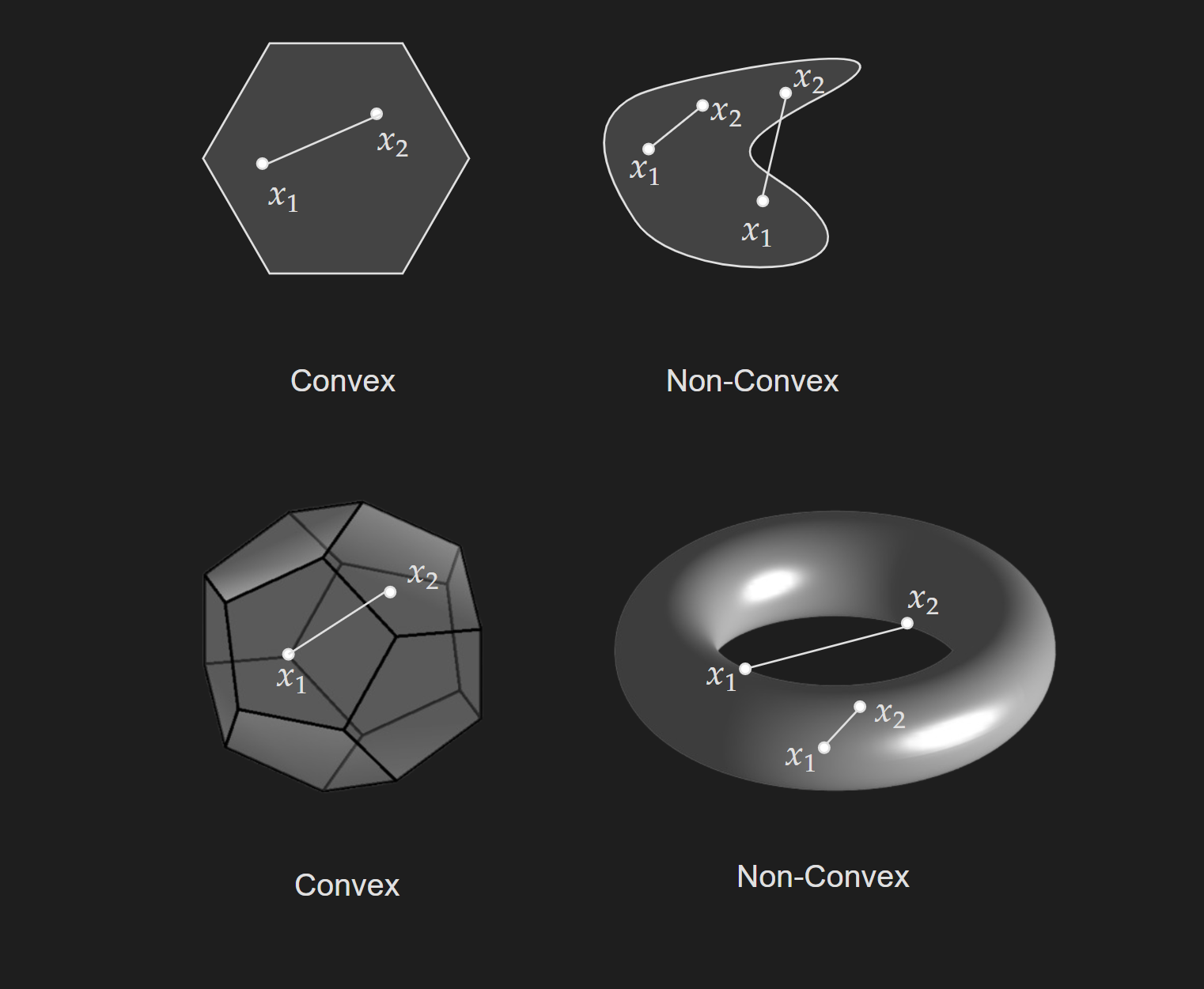
A set $C$ is convex if the line segment between any two points in $C$ lies in $C$, i.e. if for any $x_1, x_2 \in C$ and any $\theta$ with $0\leq\theta\leq 1$, we have

\[\theta x_1+(1-\theta) x_2 \in C\] \[\forall \theta \in[0,1], \forall x_1, x_2 \in C\]

Here, $\theta x_1+(1-\theta) x_2 $ represents all possible points in the line segment between $x_1$ and $x_2$ by letting $\theta$ vary.

The above picture shows a visualization of a convex set and a non-convex set in 2D and 3D. But this is a really general concept that can be easily extended to any number of dimensions.

Key Facts about Convex Sets

I will simply state some key facts about convex sets without going into rigorous proofs.

• The empty set $\emptyset$ is a convex set.

• $\mathbb{R}^{d}$ is a convex set.

• Affine transformation (scaling and translation) of a convex set produces a convex set.

• The intersection of convex sets are also convex sets.

• Hyperplanes are convex sets.

• The set $\alpha C$ is convex for any convex set $C$ and scalar $\alpha$.

Convex Functions

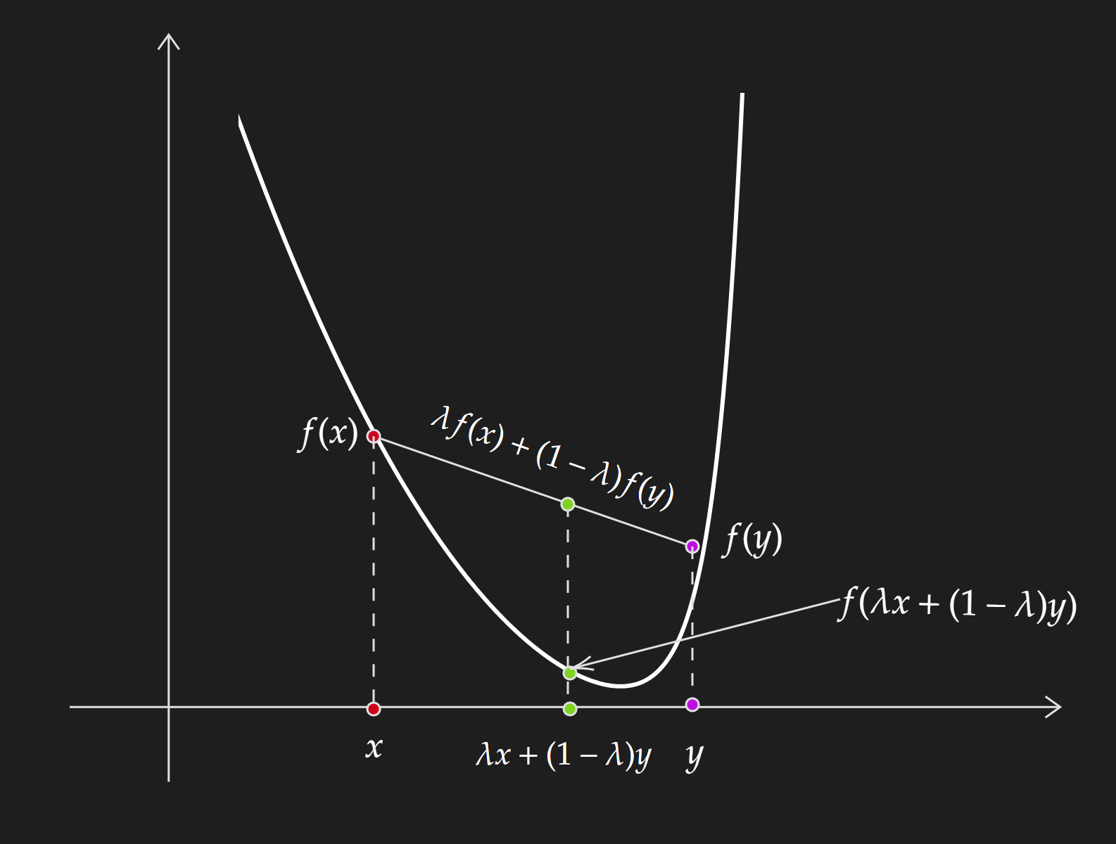
A function $f$ is a convex function if the following definition holds:

\[f(\lambda x+(1-\lambda) y) \leq \lambda f(x)+(1-\lambda) f(y)\] \[\forall~\lambda \in [0,1]\]

Look into Jensen’s inequality to get a better sense of this definition. A much simpler interpretation of this is :

The chord formed by connecting two points on the functions is above the function.

Another definition can be given with epigraph.

\[\operatorname{epi}(f)=\left\{(x, t) \mid x \in \mathbb{R}^n, t \in \mathbb{R}, \text { and } t \geq f(x)\right\}\]

In simpler terms, the epigraph of a function includes all the points that lie above or on the graph of the function. If $f$ is a convex function, its epigraph will be a convex set. Here is a nice geogebra notebook from Peter J.C. Dickinson if you want to play around with it.

Now these two definitions are actually not that useful in practice, because most of the time we deal with high-dimensional functions that we can not visualize. The way to go about it is to recognize some common convex functions (I know it sounds bad).

• $f(\mathbf{x})=\mathbf{x}^T \mathbf{A}\mathbf{x}$ is a convex function if $\mathbf{A}\succeq0$.

• $f(x)=\frac{1}{2} x^T A x+b^T x+c$ is a convex function if $\mathbf{A}\succeq0$.

• $\frac{1}{2}|X w-y|^2=\frac{1}{2} w^T X^T X w-y^T X w+\frac{1}{2} y^T y$ is convex.

Checking if the hessian (if it exists) is positive semidefinite is one of the easiest ways to check for convexity.

Key Facts about Convex Functions

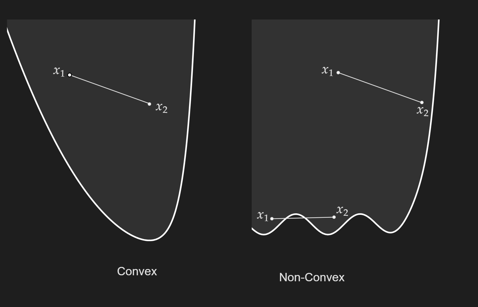
• Any local minimum is a global minimum.

• If hessian exists, the hessian is positive semidefinite.

• Level sets of convex functions are convex functions.

• The linear combination of a convex function is convex. This means $a \cdot f(x)+b \cdot g(x)$ is convex for convex $f$ and $g$ and $a,b>0$.

• $\max (f(x), g(x))$ is convex for convex $f$ and $g$.

We also need to know how to formulate a convex optimization problem.

Minimization or Maximization?

It does not matter if we need to minimize or maximize an objective function. For example suppose we need to minimize a objective function $f(\mathbf{x})$, which can be mathematically written as follows:

\[\min f(\mathbf{x})\]

This can be converted into a maximization problem as follows:

\[\max -f(\mathbf{x})\]

The other way is also true, a maximization can be converted into a minimization problem too. How an optimization problem should be posed depends on the context and the domain of the problem.

The formulation of a convex optimization problem

A standard convex optimization problem can be formed in the following way:

\[\begin{aligned} \operatorname{minimize} & f_0(x) \\ \text { subject to: } & f_j(x) \leq 0 \quad \forall j \in 1,2, \ldots, J \\ & h_k(x)=0 \quad \forall k \in 1,2, \ldots, K \end{aligned}\]

Where all $f_j(x), j \in 0,1,2, \ldots J$ are convex and all $h_k(x), k \in 1,2, \ldots, K$ are affine.

Here,

• $f_0(x)$ is the objective function.
• $f_i(x)$ are the inequality constraints.
• $h_{k}(x)$ are the equality constraints.

Some other terminology to get familiar with:

• The feasible set is the set of points that satisfy the constraints
• An inequality constraint can be in two states, active and inactive. For the values of $x$, $f_i(x)=0$, the inequality constraint is active. For the values of $x$, $f_i(x)<0$ the inequality constraint is inactive.

Another technical detail should be mentioned here. For an optimization to be convex optimization,

\[\begin{array}{ll} \operatorname{minimize} & f(x) \\ \text { subject to } & x \in C \end{array}\]

This means the feasible set needs to be a convex set.

Multivariate Calculus

Gradient

For a function $f(\mathbf{x}): \mathbb{R}^n \rightarrow \mathbb{R}$, the gradient is defined as follows:

\[\nabla f(\mathbf{x})=\frac{d f}{d \mathbf{x}}=\left(\begin{array}{c} \frac{\partial f}{\partial x_1} \\ \frac{\partial f}{\partial x_2} \\ \vdots \\ \frac{\partial f}{\partial x_n} \end{array}\right)\]

Two key things about the gradient of a function:

• The gradient points to the direction of the steepest ascent. Additionally, $-\nabla f(\mathbf{x})$ is the direction of the steepest descent.

• The gradient vectors are always orthogonal to the contour lines.

A way to think about gradients is they are a way to package up partial derivatives $ [\nabla f(\mathbf{x})]_i=\frac{\partial f(\mathbf{x})}{\partial x_i} $ in a vector form.

Hessian

For a function $f(\mathbf{x}): \mathbb{R}^n \rightarrow \mathbb{R}$, the hessian is defined as follows:

\[\nabla^2 f(\mathbf{x})=\frac{\partial^2 f}{\partial x_i \partial x_j}=\left(\begin{array}{cccc} \frac{\partial^2 f}{\partial x_1 \partial x_1} & \frac{\partial^2 f}{\partial x_1 \partial x_2} & \cdots & \frac{\partial^2 f}{\partial x_1 \partial x_n} \\ \frac{\partial^2 f}{\partial x_2 \partial x_1} & \frac{\partial^2 f}{\partial x_2 \partial x_2} & \cdots & \frac{\partial^2 f}{\partial x_2 \partial x_n} \\ \vdots & \vdots & \ddots & \vdots \\ \frac{\partial^2 f}{\partial x_n \partial x_1} & \frac{\partial^2 f}{\partial x_n \partial x_2} & \cdots & \frac{\partial^2 f}{\partial x_n \partial x_n} \end{array}\right)\]

According to Schwarz’s Theorem, the hessian is symmetric if it exists, that is :

\[\frac{\partial^2 f}{\partial x_i \partial x_j}=\frac{\partial^2 f}{\partial x_j \partial x_i}\]

Taylor Series Approximation

The best way to think about the Taylor series is it approximates non-linear functions with piece-wise terms. Which is a lot easier to think about in one dimension. Go through this video from 3blue1brown to appreciate the Taylor series in one dimension.

You need to extrapolate this intuition in higher-dimension (at least for $f:\mathbb{R}^2 \rightarrow \mathbb{R}^3$) which is not an easy task. Usually, we never use more than 2nd-order terms in Taylor series expansion.

\[f(\mathbf{x}+\Delta \mathbf{x})=f(\mathbf{x})+\sum_i \frac{\partial f(\mathbf{x})}{\partial x_i} \Delta x_i+\frac{1}{2} \sum_i \sum_j \frac{\partial^2 f(\mathbf{x})}{\partial x_i \partial x_j} \Delta x_i \Delta x_j+\cdots\]

A more concise way to write this is as follows:

\[f(\mathbf{x}+\Delta \mathbf{x})=f(\mathbf{x})+\nabla f(\mathbf{x})^{\mathrm{T}} \Delta \mathbf{x}+\frac{1}{2} \Delta \mathbf{x}^{\mathrm{T}} \nabla^2 f(\mathbf{x}) \Delta \mathbf{x}+O\left(\|\Delta \mathbf{x}\|^3\right)\]

where, $O\left(|\Delta \mathbf{x}|^3\right)$ are the higher order terms.

Now, sometimes we write $\mathbf{z}=\mathbf{x}+\Delta \mathbf{x}$ which is considered as another point in the graph. Note that, $\mathbf{z}-\mathbf{x}=\Delta \mathbf{x}$. Therefore, the above expression can be rewritten as follows:

\[f(\mathbf{z})=f(\mathbf{x})+\nabla f(\mathbf{x})^{\top}(\mathbf{z}-\mathbf{x})+\frac{1}{2} (\mathbf{z}-\mathbf{x})^{\top} \nabla^2 f(\mathbf{x}) (\mathbf{z}-\mathbf{x})+O\left(\|\Delta \mathbf{x}\|^3\right)\]

If we consider only the first-order term,

\[f(\mathbf{z})\approx f(\mathbf{x})+\nabla f(\mathbf{x})^{\mathrm{T}}(\mathbf{z}-\mathbf{x})\]

Be careful about how interpret it. We are not performing Taylor series approximation at $\mathbf{z}$, we approximating it “around” point $\mathbf{x}$ and the returned expression will contain $\mathbf{z}$ terms.

Sometimes it gets so confusing that; people use different notating to make it explicit.

\[f(\mathbf{x})=f\left(\mathbf{x_0}\right)+\nabla f\left(\mathbf{x_0}\right)^{\top}\left(\mathbf{x}-\mathbf{x}_0\right)+\frac{1}{2}\left(\mathbf{x}-\mathbf{x_0}\right)^{\top} \nabla^2 f\left(\mathbf{x_0}\right)\left(\mathbf{x}-\mathbf{x_0}\right)+\text{higher order terms}\]

Supremum and Infimum

This is a “hard” concept to get your head around. Sometimes to avoid rigorous definitions, supremum is replaced with “max” and infimum is replaced with “min”. This is fine as long as your optimization problem is “nice” and “well-behaved”. Therefore, there is a good chance you can get away with just “min” and “max”. But most of the resources you will come across, prefer “supremum” and “infimum” to enforce mathematical rigor. The definitions I will provide below are by no means a complete definition; because you can always argue about the “rigorousness” of the definition, but they should be enough to understand their usage in convex optimization.

Supremum

For a subset $S \subseteq \mathbb{R}$, $u \in \mathbb{R}$ is called an upper bound for $S$ if

\[\forall x \in S: x \leq u\]

Note that, we did not say $u \in S$, because the definition is more general. $u$ might or might not be in the set, meaning the definition holds whether $u \in S$ or $u \notin S$.

If $u$ is an upper bound for $S$ and $u \in S$, then $u$ is called the maximal(or max) element of $S$. This is pretty easy to get your head around. Consider a set $S={ 1, \frac{1}{2}, \frac{1}{4} }$. We can easily say $u=1$ is the maximal element because $u$ is the upper bound for the set and also an element of the set.

But people get confused by the other case which is $u$ is an upper bound of $S$, but not an element of $S$ i.e. $u \notin S$. Consider $S=(0,1)$. Here the upper bound of the set is $1$. Technically, this is wrong, because $4$ is also another upper bound, so is $5$ and so on. The correct term to use here is $1$ is the “least upper bound” for $S=(0,1)$. Note that even though it is the least upper bound it is not an element. The values of set $S$ will get really really close to $1$, but will not include $1$.

From this, we can define the supremum. For a non-empty subset $S \subseteq \mathbb{R}$ (which needs to be upper bounded, yes it is possible to have unbounded sets), $u \in \mathbb{R}$ is called supremum of $S$ if $\forall x \in S: x \leq u$ and if $M$ is an upper bound of $S$, then $u\leq M$. It is written as:

\[\sup (S)=u \Longleftrightarrow(\forall x \in S, x \leq u) \wedge(\forall M \text { upper bound of } S, u \leq M)\]

Just for the sake of completeness, we need to know two additional facts.

• If $S$ is non-empty and $\textbf{not}$ bounded above, then,

\[\sup (S)=\infty\]

• If $S=\emptyset$, then

\[\sup (S)=-\infty\]

Infimum

For a subset $ S \subseteq \mathbb{R} , l \in \mathbb{R} $ is called a lower bound for $S$ if

\[\forall x \in S: x \geq l\]

If $l$ is a lower bound for $S$ and $l \in S $, then $l$ is called the minimal (or min) element of $S$. For infimum, we need the “largest lower bound”. This is formally defined as follows given $S$ is a non-empty set and bounded below:

\[\inf (S)=l \Longleftrightarrow(\forall x \in S, x \geq l) \wedge(\forall N \text { lower bound of } S, l \geq N)\]

Again for the sake of completeness, we need to know two additional facts.

• If $S$ is non-empty and $\textbf{not}$ bounded below, then,

\[\inf (S)=-\infty\]

• If $S=\emptyset$, then

\[\inf (S)=\infty\]

Subgradient and Subdifferentials

Subgradient

Subgradients are a generalization of gradients for both differentiable and non-differential functions. I will directly write down the definition from Boyd,

A vector $g \in \mathbb{R}^n$ is a subgradient of $f:\mathbb{R}^n \rightarrow \mathbb{R}$ at $x \in \textbf{dom} f$ if for all $z \in \textbf{dom} f$

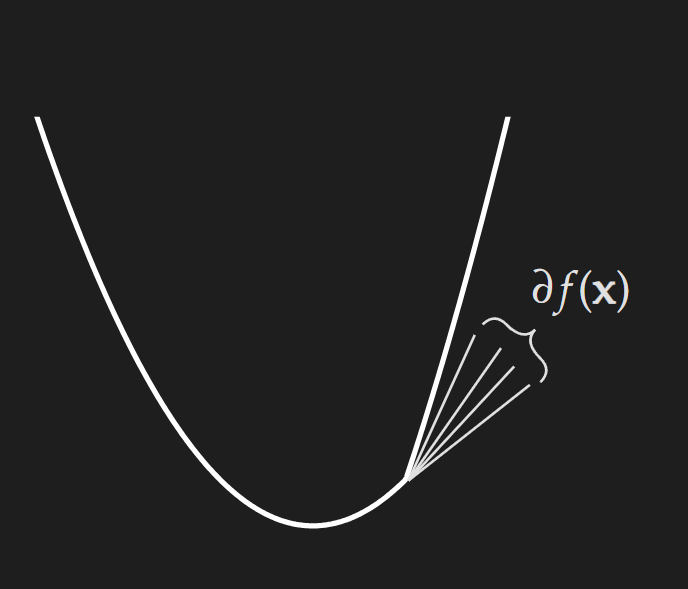
\[f(z) \geq f(x)+g^T(z-x)\]

As an example, consider the following function:

\[f(\mathbf{x})= |x_1 -2|+(x-1)^2\]

The plot of the function is given below:

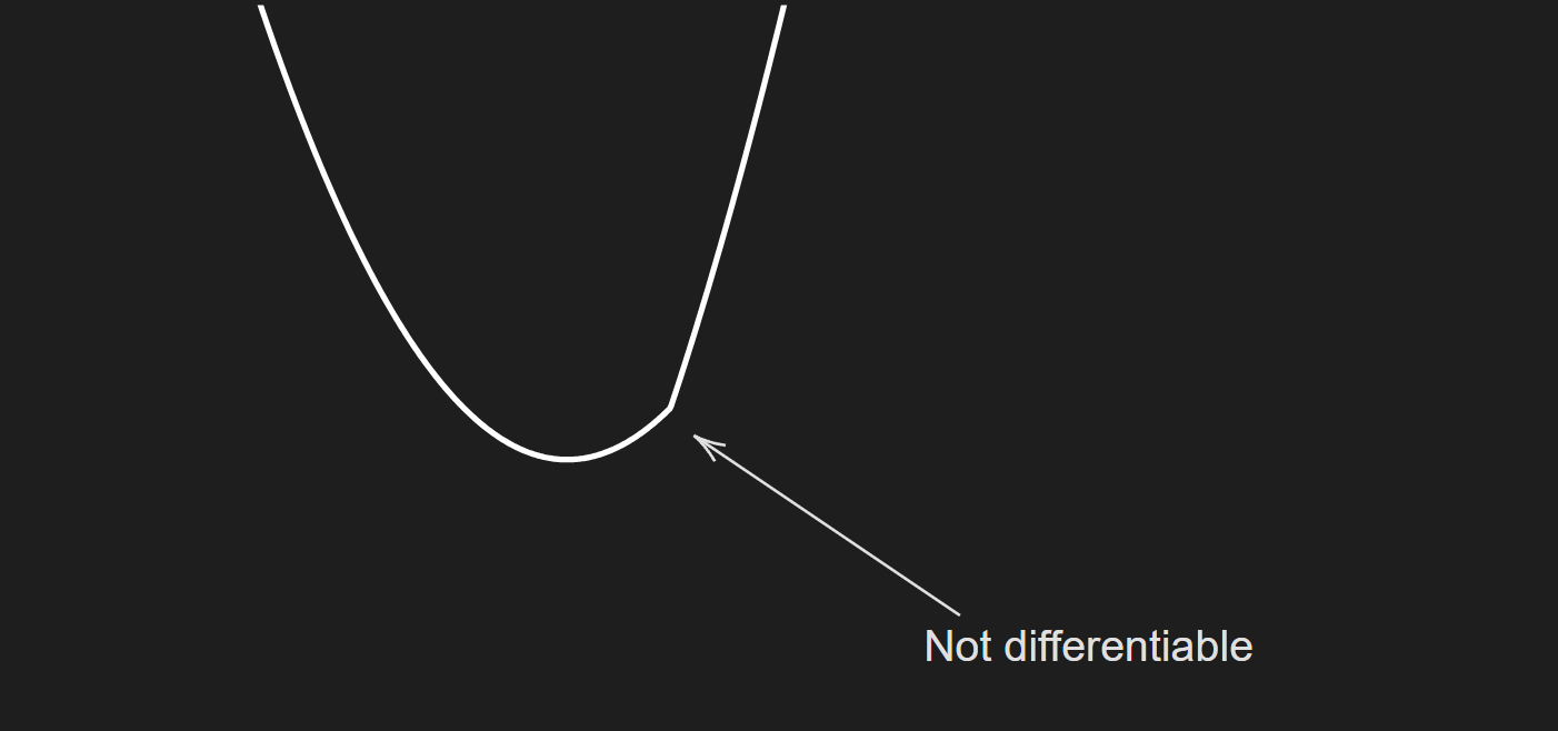
A visualization of some possible subgradient at the non-differentiable point is given below:

Subdifferentials

The set of subgradients of $f$ at the point $x$ is called the subdifferential of $f$ at $x$ and is denoted by $\partial f(x)$.

\[\partial f(x)=\left\{g \in \mathbb{R}^n \mid f(z) \geq f(x)+g^T(z-x), \forall z \in \mathbb{R}^n\right\}\]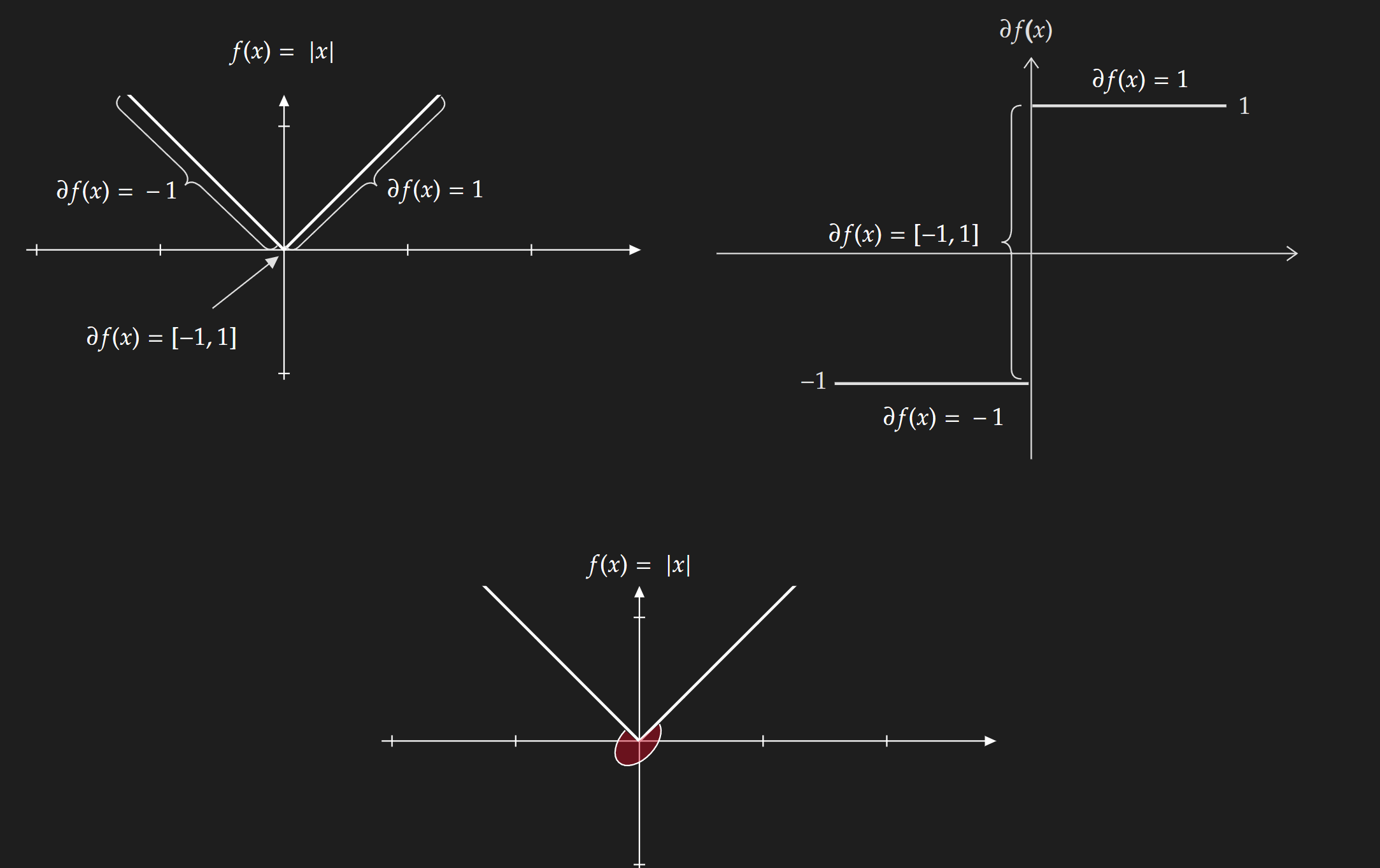

For differentiable convex functions, this set contains only one element which is the gradient of the function at point $x$. Mathematically,

\[\partial f(x) = \{ \nabla f(x)\}\]

I highly encourage interested readers to go through the lecture notes from Boyd.