Moving Beyond OLS-Introduction to GLMs
In this article, I am going to give a beginner-friendly introduction to generalized linear models (GLMs). As a prerequisite, you should have a pretty clear idea about about OLS and the assumptions of OLS. Also, you need to be somewhat familiar with the exponential family of distributions.
Generalized Linear Models (GLM)
This starts with the idea about the ordinary least squares (OLS) and the assumptions we make when we fit an OLS. One of the assumptions is the response variable follows a Gaussian distribution with constant variance. When we are introduced to OLS we come across a figure like the following:
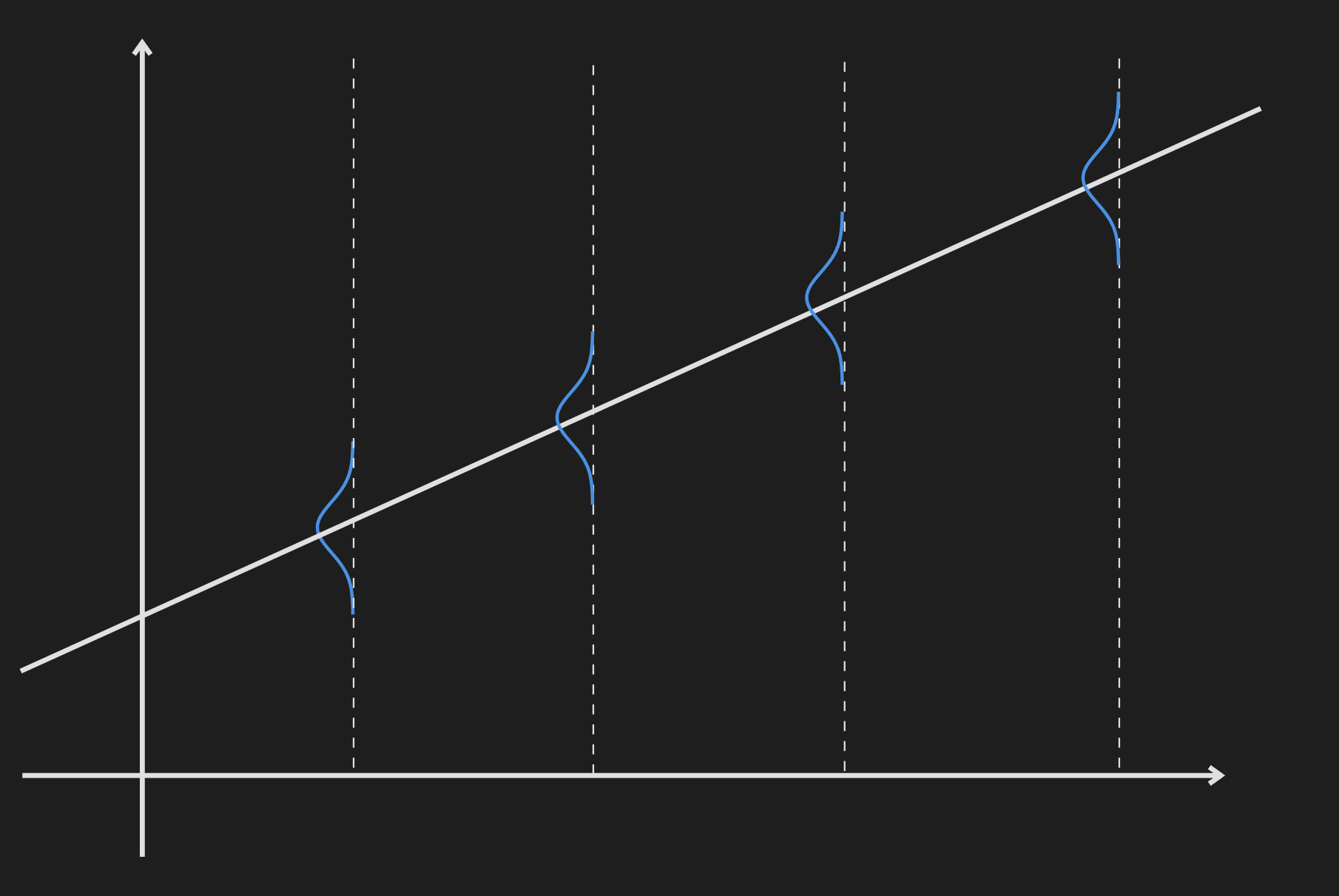
In this figure, the Gaussian distribution of the response variable is superimposed on the regression line.
To get a better perspective we can look at it from another perspective:
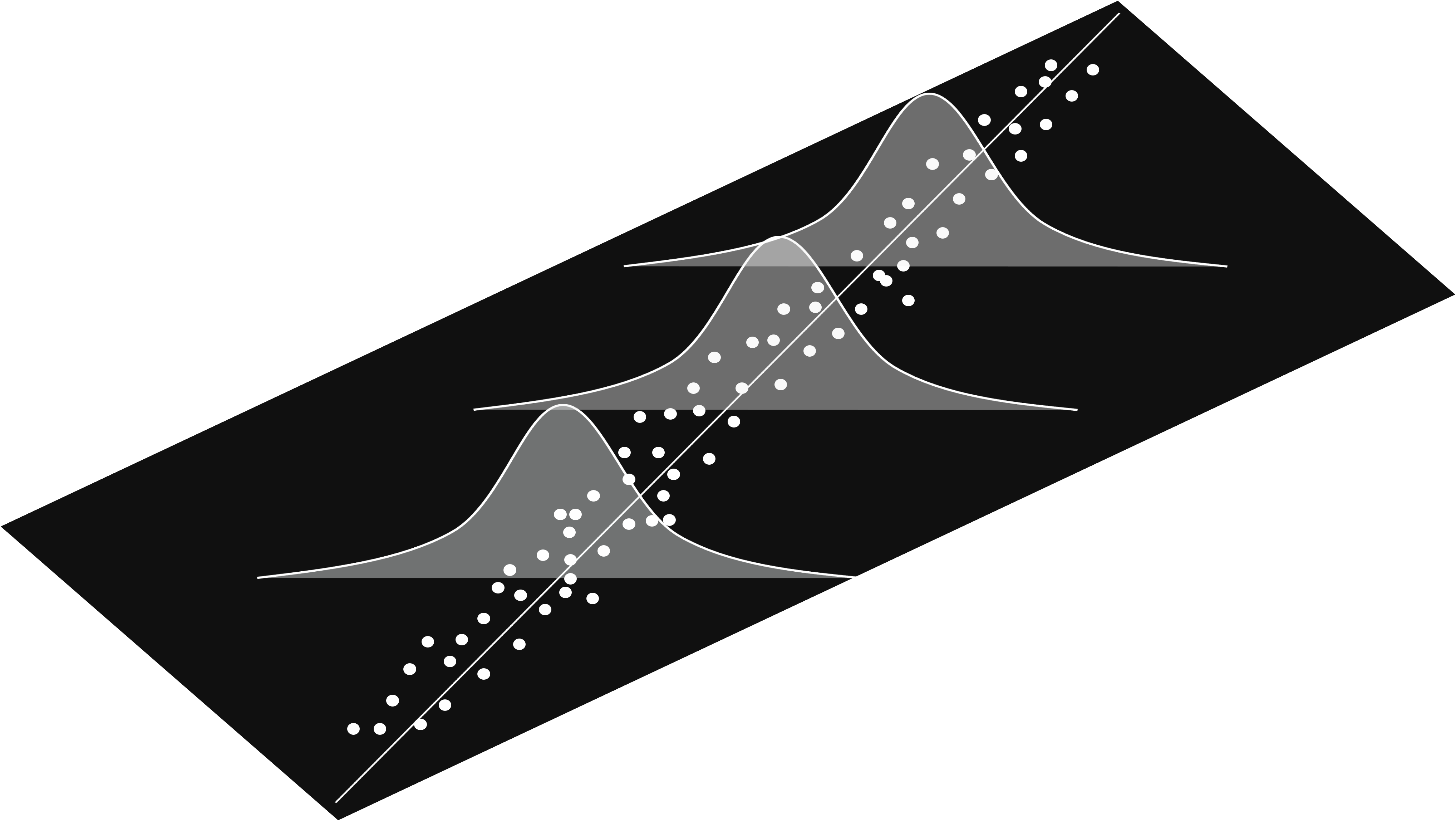
I think anyone can immediately see the problem if this model is to be applied in a real-world scenario. The response variable is not always going to follow the Gaussian distribution. When it does not follow a Gaussian distribution the OLS is going to fail. Also for OLS to work it needs to abide by the homoscedasticity requirement which is often not the case in real-life data.
How do we adjust for this? Is there a way we can specify the distribution of the response variable beforehand and the model will adapt accordingly? Generalized linear models do exactly that. A well-known example of GLM is logistic regression where we assume the response variable follows a Bernoulli distribution.
There are three components related to a generalized linear model.
Systemic Component: This is the component that contains the predictor variables $x_1,x_2,x_3,\cdots,x_n$. This means the systemic component is $\beta_0+\beta_1x_1+\beta_2x_2+\cdots+\beta_nx_n$.
Random Component: This is the probability distribution of the response variable. For OLS this is a Gaussian distribution, for binary logistic regression this is a Binomial distribution. As these are related to distributions, they act as random components in the model.
Link Function: It is typically denoted by $\eta$ or $g(\cdot)$. The link function connects the random component and the systemic component. The general formula for link functions is given by the following:
This signifies the link function connects the expected value of the response variable to the linear combination of predictor variables.
For OLS the link function is just an identity mapping meaning $\eta=g(E(Y_i))=E(Y_i)$. This makes sense, because for Gaussian distribution the expected value of the response variable is in the center of the distribution.
For binary logistic regression, the link function is the logit function.
Some people might get confused about the expectation term appearing out of nowhere. Let’s take a closer look at OLS:
\[\mathbf{Y}=\mathbf{X}^{T} \mathbf{\beta}+\epsilon\]we assume $\epsilon\sim\mathcal{N}(0,\sigma^2\mathbf{I})$. It is possible to absorb the $\epsilon$ directly in our model. This turns $\mathbf{Y}$ into a random variable which follows a conditional distribution as follows:
\[\mathbf{Y}|\mathbf{X} \sim \mathcal{N}(\mathbf{X}^{T} \mathbf{\beta},\sigma^2\mathbf{I})\]From the above equation, we can see how for an OLS the expectation of response variables $\mathbf{Y}$ relates to the linear combination of predictor variables. The above equation can also be written as follows:
\[\mathbf{Y}|\mathbf{X} \sim \mathcal{N}(\mu(\mathbf{X}),\sigma^2\mathbf{I})\]where, the expectation is a general function of $\mathbf{X}$ expressed as $\mu({\mathbf{X}})$. In OLS, we assume $\mu({\mathbf{X}})$ is directly equal to $\mathbf{X}^{T}\beta$, but for GLM this assumption is relaxed. More precisely,
\[\mu(\mathbf{X})= f(\mathbf{X}^{T}\beta);~\text{where}~f(\cdot)=g^{-1}(\cdot)\]The above equation can be written in terms of link function $g(\cdot)$ as follows:
\[g(\mu(\mathbf{X}))= \mathbf{X}^{T}\beta\]One important detail everyone forgets to mention is, that the GLM only works if the distribution of the response variable is from the exponential family. Exponential family is defined generally in the following form:
\[f(y|\theta, \phi) = \exp\left\{\frac{t(y)\theta - b(\theta)}{a(\phi)} + c(y, \phi)\right\}\]I am not going to go into details about exponential family in this article, you will have to take my word for it. This can help us give a concise definition of the GLMs.
IN GLMs, the response variable $y_i$ follows a distribution from the exponential family with an expected value of $\mu_i$. This expected value $\mu_i$ can be modeled as a function of the linear combination of response variables. But this is not necessarily a direct functional mapping but a mapping after applying the link function.
One common doubt about generalized linear models is, why they are called linear if they are modeling non-linear relationships between the response and predictor variables. The answer to that is the model is linear in parameter.
Another common confusion about generalized linear models is the interpretation of link functions. Why do we even need a link function? There are several explanations for this. One explanation that seems the most intuitive to me is it makes $\mu(\mathbf{X})$ and $\mathbf{X}^{T}\beta$ compatible. For example, if your response variable is restricted to strictly non-negative numbers, the link function should transform $\mu_i$ to a non-negative number. But this raises another issue. Based on this requirement there is a plethora of possible link functions. How do we choose the best one? Here comes the idea of canonical link functions. You can think of canonical link functions as the default choice for link functions if you have no idea about choosing the link functions. Note that, it is not necessary to use the canonical link function, and if you have domain knowledge about the problem at hand and think another link function will work better, the canonical link function can be ignored.
You can find a nice summary of the distributions and link functions in Wikipedia. Also, for a nice visual introduction, you can refer to this video.