Lagrange Multipliers

Lagrange multipliers is a general concept in optimization theory that is applicable to any high dimensional surface. The drawback with such generalization is we can not visualize more than 3 dimensions. But it is possible to have some intuitions in the low-dimensional space and those intuitions do carry over to higher dimensions.

To fully appreciate Lagrange multipliers, some pre-requisite concepts must be understood.

Contour Lines

Consider the following function which is given by the equation

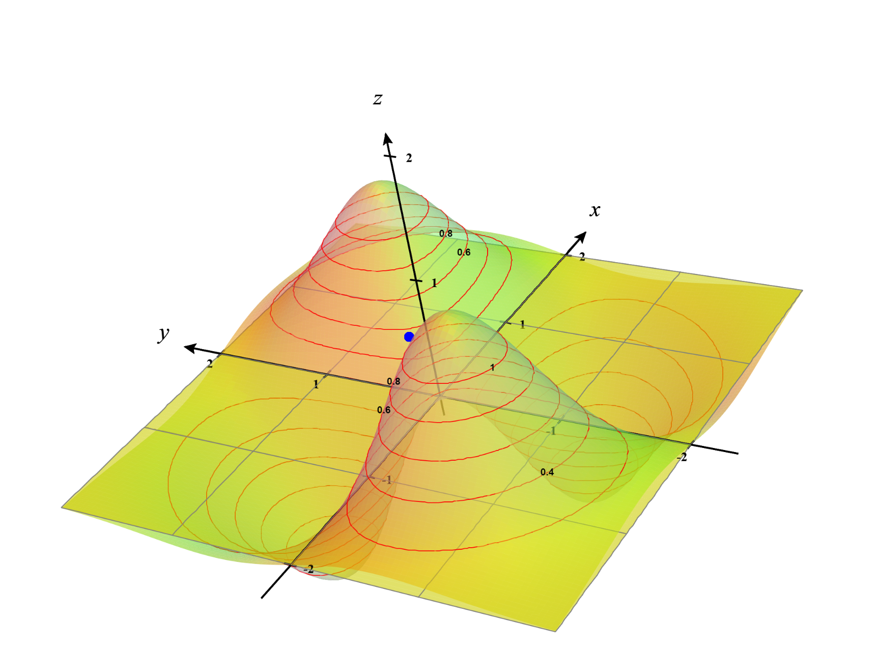
\[f(x,y)=\frac{7xy}{e^{x^2+y^2}}\]

A 3-dimensional visualization of the function is shown below:

We can draw contour lines in the 3D surface of the plot which is shown below:

A better way to see these contour lines is a contour plot generated from the top-down perspective as shown below:

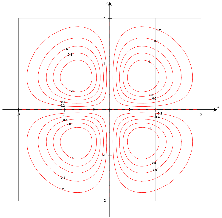
Think of it as the contour lines being projected to the x-y plane. See the below plot as a reference. I removed the original graph and kept only the contour lines. The Contour lines in the 3D surface are colored in green and the projected version in the x-y plane is colored in red.

I hope after seeing these visualizing contour plots are more intuitive now.

Gradient vectors are orthogonal to contour lines

One special thing about contour lines is the gradient vectors of the function $f(x,y)$ i.e. $\nabla f(x,y)$ are always orthogonal to contour lines. This can be easily understood with the hill-climbing analogy. Imagine the surface in our discussion as some terrain we are trying to traverse.

What happens when we walk along the contour lines?

• Do we climb up?
• Do we climb down?
• Do we stay on the same level?

The answer is we stay on the same level by definition of contour lines. That means walking along the contour lines has a contribution of “0” if we want to climb the hills as fast as possible.

Now consider these three facts side by side :

• Walking along the contour lines contributes “0” to climbing the hill

• That means moving in the orthogonal direction contributes “maximum” to climbing the hill. Meaning that you want to climb in that direction which does not have any component in the direction of the contour lines. Because that “component” along the contour line is getting wasted as it contributes “0” to the hill-climbing. Walking orthogonal to contour lines means there is no component whatsoever along the contour lines.

• Gradient vectors show the direction of the steepest ascent.

Voila! This means gradient vectors are always orthogonal to the contour lines.

Adding a Constraint Curve

Now if we do not want to find the maximum of the function at any given point, rather along a curve we define, the optimization problem turns into a constrained optimization. To start, let us introduce a single constraint curve. To keep it simple, we will consider a unit circle center at the origin,

\[x^2+y^2=1\]

From the contour plot perspective, it looks like the following:

If we look back a the 3D surface we will get something like the following:

If we visualize the portion of the function $f(x,y)$ under the constraint, we get something like the following:

If we change our constraint curve from $x^2+y^2=1$ to $x^2+y^2=3$ this visualization changes to the following:

We can see how the constraint curve changes the maxima and minima location of the function under constraint.

Constraint Curve Gradient

Now we can define the constraint curve (surface) as follows:

\[g(x,y)= x^2+y^2\]

Wait a minute this is not a curve in the 2D x-y plane! This is the equation of a surface. Well, that’s correct. And that surface looks like the following:

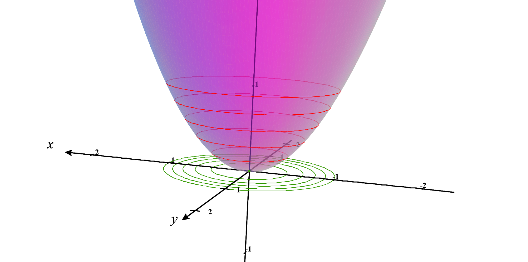
But take a closer look at the contour lines for this surface. Each contour line is a circle. The first constraint curve we considered is one of those contour lines. The second constraint curve also.

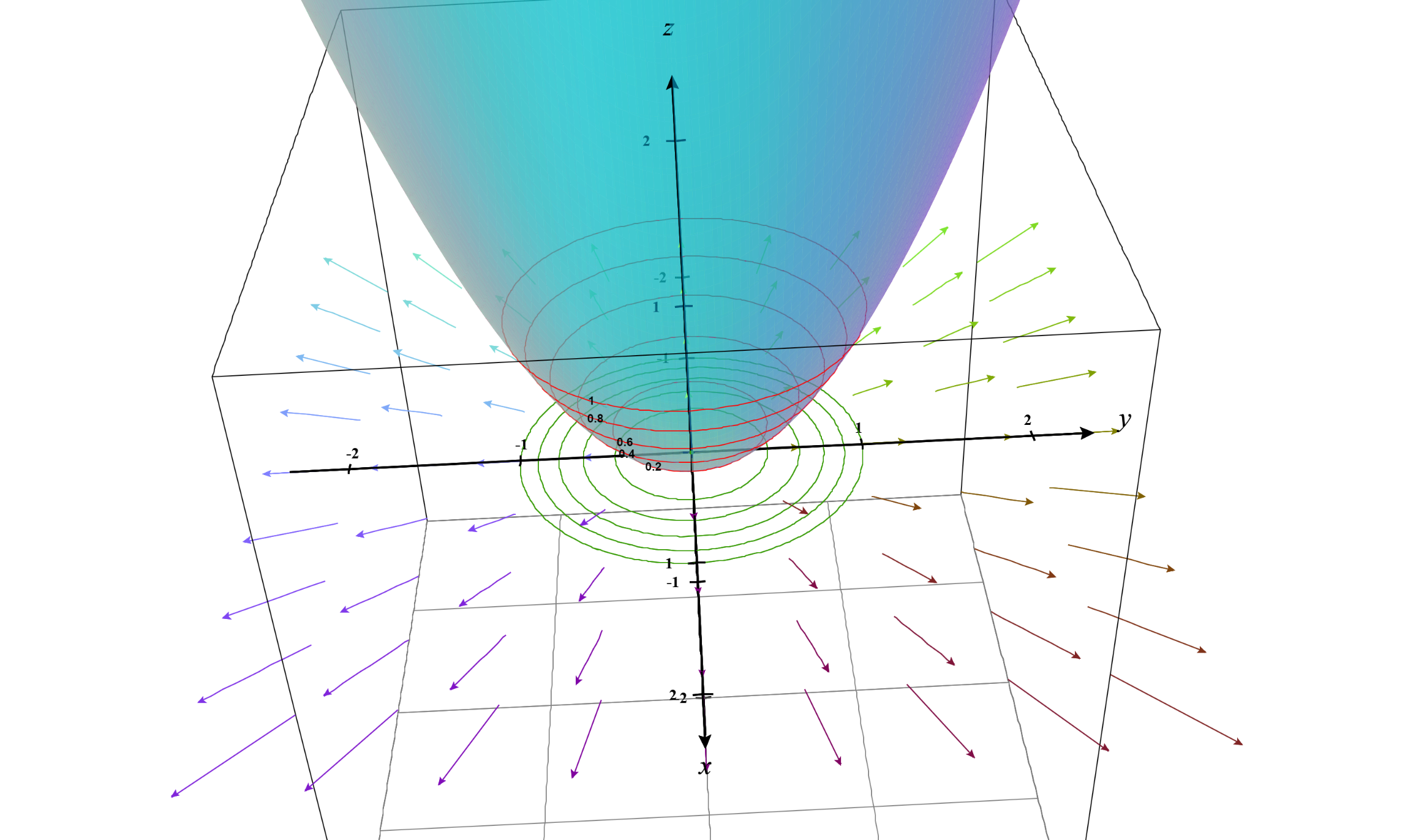
If we take the gradient of that surface we get $\nabla g(x,y)$. Now if you think about it the gradient vector of $g(x,y)$ is also perpendicular to the contour lines.

A 3D visualization is given below:

We can also take a look from the contour plot perspective as follows:

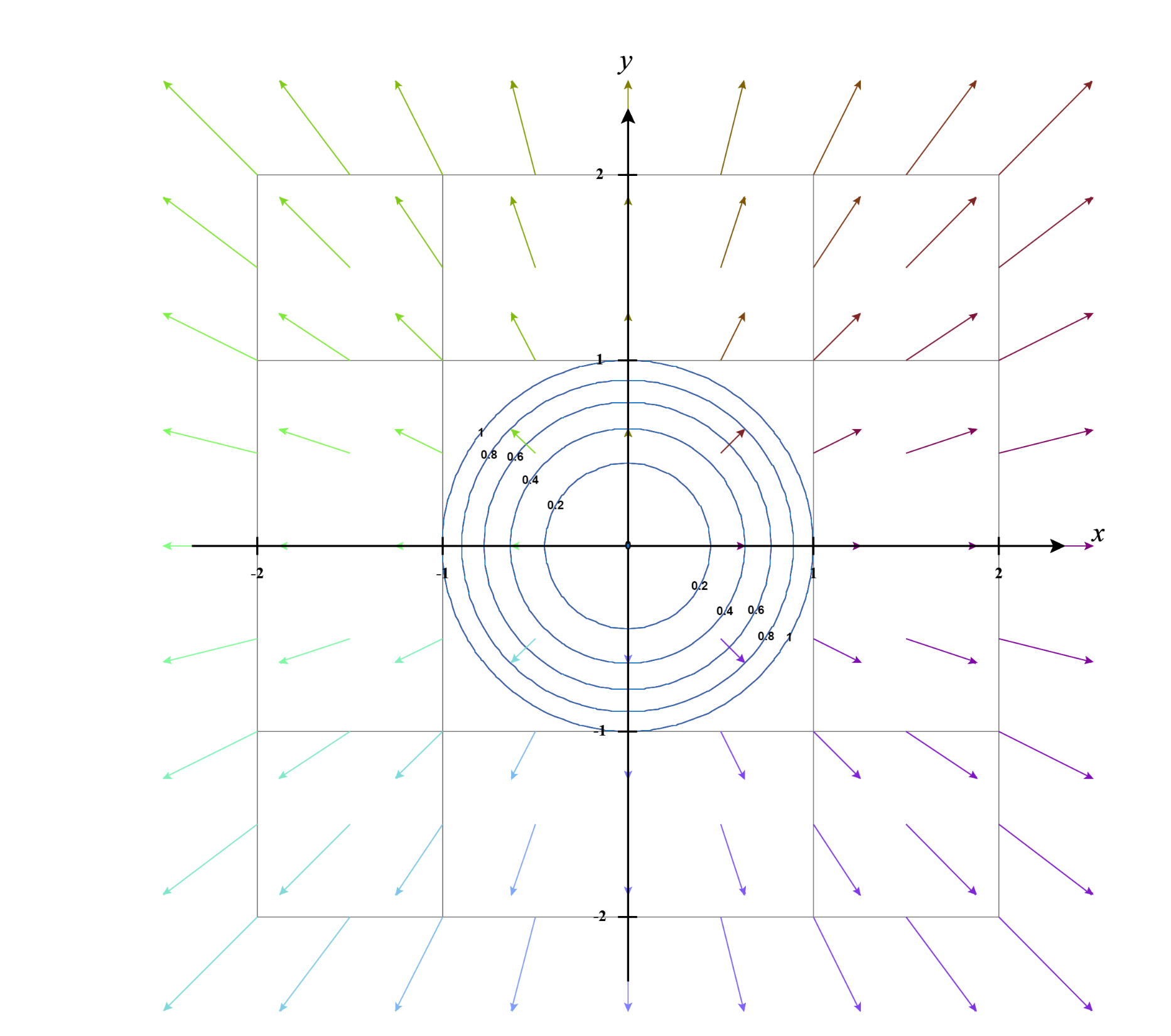
This means $\nabla g(x)$ and $\nabla f(x)$ are parallels!

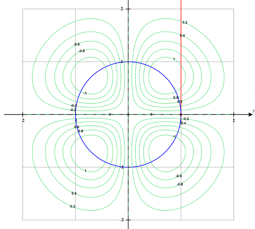
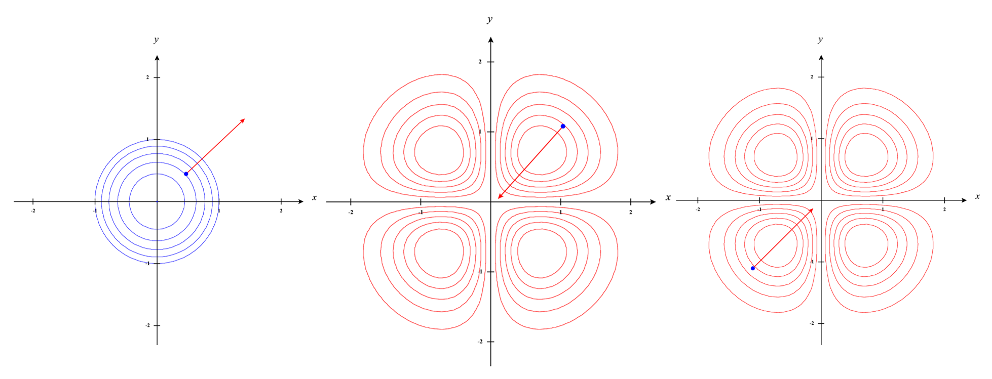
Visually, if we want to see it we can plot the contour lines of $f(x,y)$ and $g(x,y)$ in a single plot.

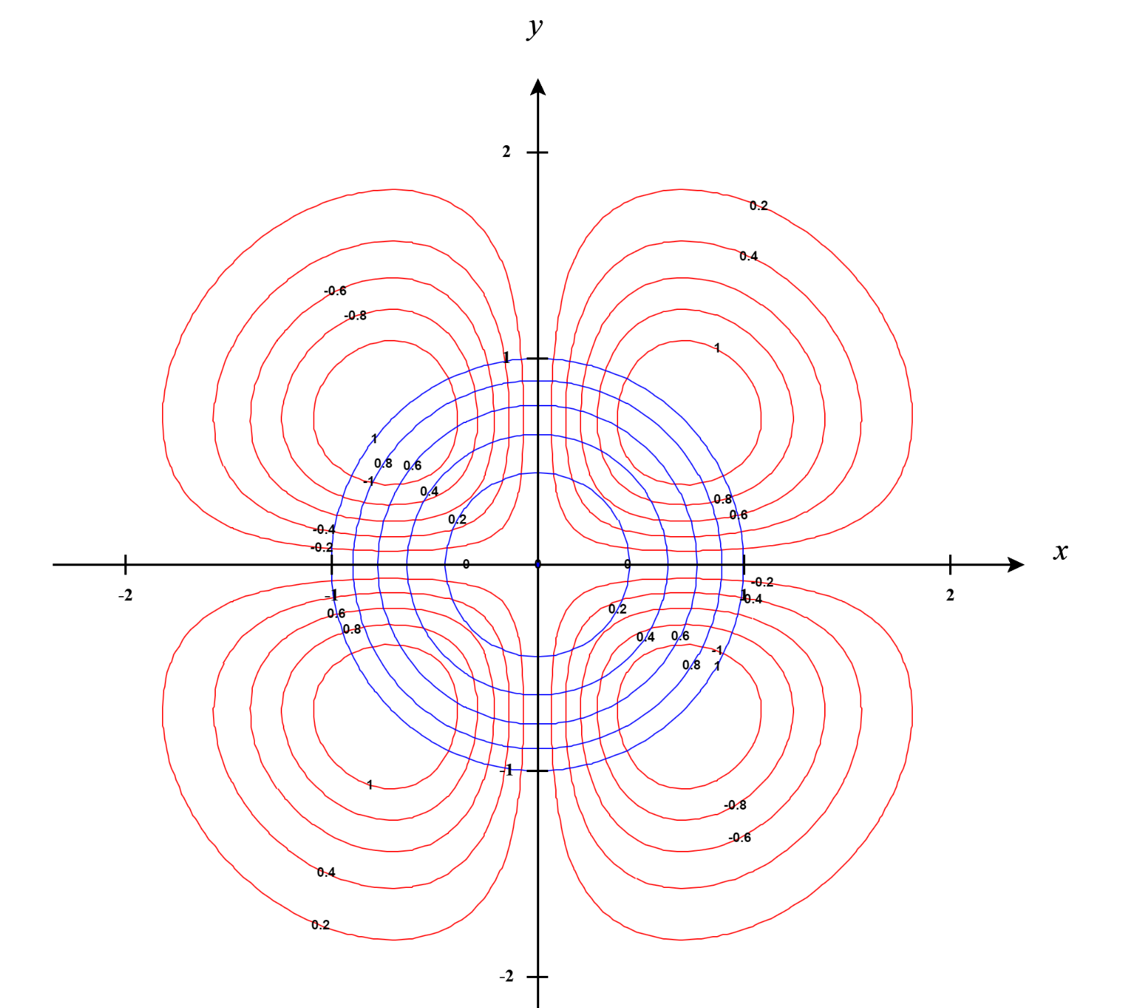
In the above plot, the blue lines are the contour plots of $g(x,y)$ and the red lines are the contour plots $f(x,y)$. Now let’s see the gradient vector at the contour lines which are plotted below. Well, just as we assumed, the gradient vectors are parallel. Note, the word “parallel”. We are not saying they are in the same direction.

If $\nabla f(x,y)$ and $ \nabla g(x,y)$ are parallel we can multiply a scalar with $ \nabla g(x,y)$ to make it equal to $\nabla f(x,y)$.

A visualization of a gradient vector on a specific contour line for $f(x.y)$ and $g(x,y)$ is given below:

The Lagrange Multiplier

\[\nabla f(x,y) = \lambda \nabla g(x,y)\]

where $\lambda$ is a scalar value which scales the gradient vector $\nabla g(x,y)$. And this $\lambda$ is the Lagrange multiplier.

Now suppose, we go through the computation.

\[\nabla f(x,y)= \left[ \begin{aligned} \frac{ \partial f(x,y)}{\partial x} \\ \frac{ \partial f(x,y)}{\partial y} \end{aligned} \right]\] \[\nabla g(x,y)= \left[ \begin{aligned} \frac{ \partial g(x,y)}{\partial x} \\ \frac{ \partial g(x,y)}{\partial y} \end{aligned} \right]\]

We get two sets of equations,

\[\frac{ \partial f(x,y)}{\partial x}= \lambda \frac{ \partial g(x,y)}{\partial x}\] \[\frac{ \partial f(x,y)}{\partial y}= \lambda \frac{ \partial g(x,y)}{\partial y}\]

But we have three unknowns $x$, $y$ and $\lambda$. The third equation will be the equality constraint itself $x^2+y^2=1$.

Now we can be smart and avoid this dependence on the third equation. We can redefine our constraint function as $x^2+y^2-1=0$. And swap sides for the original equations:

\[\nabla f(x,y) - \lambda \nabla g(x,y)=0\]

Now, we can let the negative sign get absorbed in the Lagrange multiplier and rewrite the equation as follows:

\[\nabla f(x,y) + \lambda \nabla g(x,y)=0\]

This can be re-written as the following:

\[\nabla (f(x,y) + \lambda g(x,y))=0\]

Note that, $ \mathcal{L}(x,y,\lambda)=f(x,y) + \lambda g(x,y)$ is referred to as the Lagrangian which is nothing but a unified equation for the objective function and the constraints.

This can be interpreted as we take the partial derivative with respect to $x$, $y$ and $\lambda$ and get the three sets of equations:

\[\frac{\partial f(x,y)}{\partial x}+\lambda \frac{\partial g(x,y)}{\partial x}=0\] \[\frac{\partial f(x,y)}{\partial y}+\lambda \frac{\partial g(x,y)}{\partial y}=0\] \[g(x,y)=0\]

Notice that to form the third equation we took the partial derivative with respect to $\lambda$ and actually got back the constraint equation itself. And, the first two equations essentially remain the same just with an additional negative sign which is the side effect of having $\lambda$ absorb the negative sign before. That means we solving the exactly same problem as before.

The mathematical convenience of this approach is we are dealing with a single equation that includes both the objective function and the constraint. Another convenience is we can use the same mathematical tool for solving constrained optimization problems that we used for unconstrained optimization problems. By that, I mean we are using gradients and first-order partial derivatives.

Generalizing the approach for Multi-Constraint Objective

Just as a caution this approach is for equality constraints. Inequality constraints are not considered here. We can collect all the equality constraints and write them in a vector format $g(\mathbf{x})$. For each equality constraint, there will be a Lagrange multiplier. We also collect these into a vector $\mathbf{\lambda}$. The modified Lagrangian can be written as the following:

\[\nabla \mathcal{L}(\mathbf{x},\mathbf{\lambda})=f(\mathbf{x})+\mathbf{\lambda}^{\top}g(\mathbf{x})\]

Where, $\mathbf{x}=\left[ \begin{aligned} x_1 \ x_2 \ . \ . \ . \ x_n \end{aligned} \right]^{\top}$, $\mathbf{\lambda}=\left[ \begin{aligned} \lambda_1 \ \lambda_2 \ . \ . \ . \ \lambda_n \end{aligned} \right]$. To be clear about notation, I always consider vectors as column vectors.

Then we take the gradient of the Lagrangian to compute $\nabla \mathcal{L}(\mathbf{x},\mathbf{\lambda})$ and set them equal to zero vector: $\mathbf{0}=\left[ \begin{aligned} 0 \ 0 \ . \ . \ . \ 0 \end{aligned} \right]^{\top}$.