Jensen's Inequality
The Basic Idea
Jensen’s inequality requires prerequisite knowledge about the definition of convex functions. I will assume the readers are somewhat familiar with convexitiy of functions.
Jensen’s inequality is one of most fundamental concept which connects a lot of different ideas in information theory. Most of things we taken for granted in information theory or hand-wave with intuition are proved with Jensen’s inequality.
The statement says that given a real-valued convex function $f(\cdot)$ and a random variable $X$ the following inequality relation holds true:
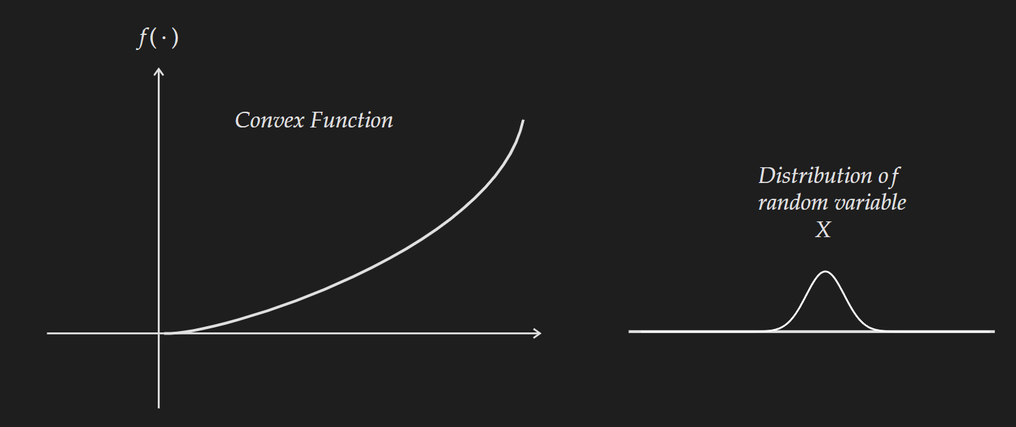
\[f(\mathbb{E}[X]) \leq \mathbb{E}[f(X)]\]There are two components to this inequality relation. The first component is a convex function $f(\cdot)$ and another is a random variable $X$. Now as we are dealing with a random variable there has to be distribution associated with it. There is no restriction on what kind of distribution it could be. For the purpose of visualization, I chose normal distribution.
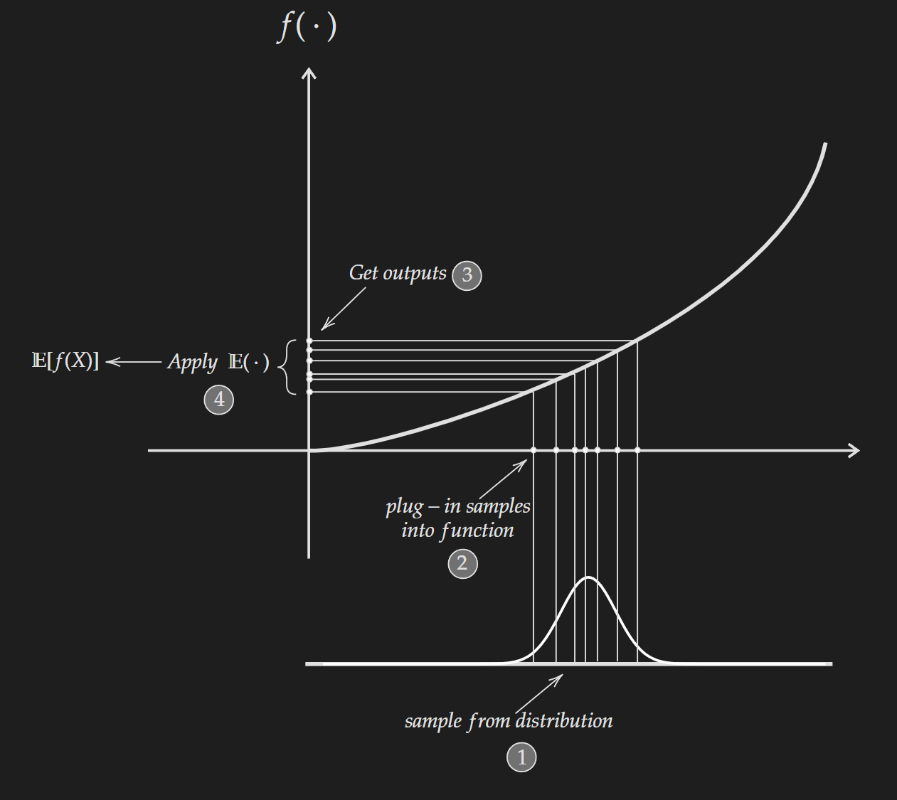
Right Hand Side : $\mathbb{E}[f(X)]$
To get this quantity we need to sample from the distribution associated with $X$ and plug them into the convex function $f(\cdot)$ and we will get outputs $f(X)$. Then we apply expectation to get $\mathbb{E}[f(x)]$.
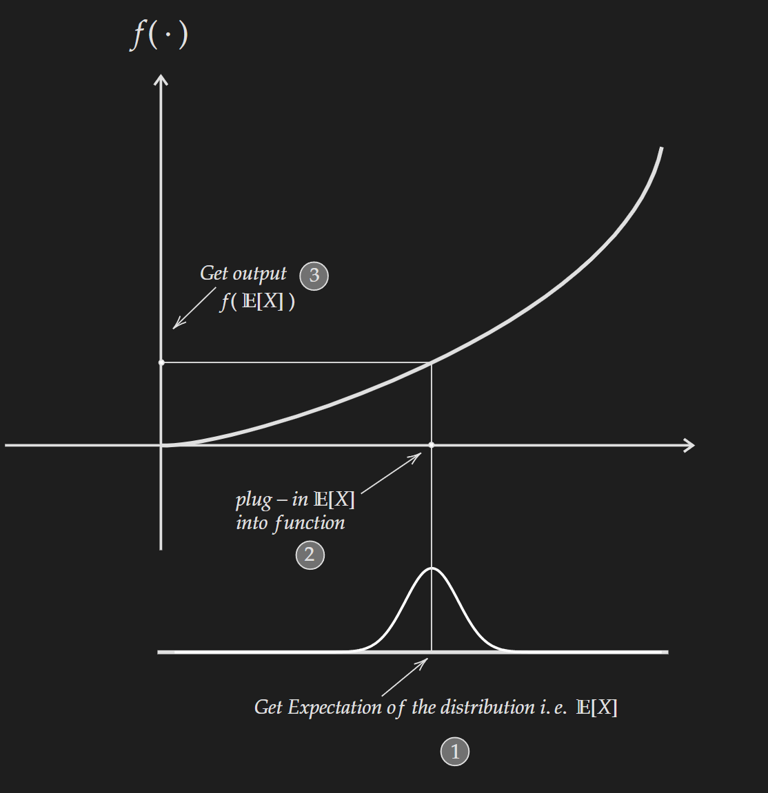
Left Hand Side : $f(\mathbb{E}[X])$
To get this quantity we first compute the expectation of the random variable to get $\mathbb{E}[X]$. Then we plug that into the convex function $f(\cdot)$ to get $f(\mathbb{E}[X])$.
One thing to note here, this holds for any number of sample points (more than one) and for any number of dimensions.
Application of Jensen’s Inequality
Well there are numerous application, but to keep it concise I will provide two such application. One is in the proof of non-negativity of KL divergence. Another is it’s usage in the wild, a research paper related to explainability in graph neural network.
To Prove the Non-Negativity of KL Divergence
For this proof first we need to know the fact that $- \log$ is a convex function. Now let’s start with the definition of KL divergence and do some algebraic manipulations.
\[\begin{align*} D_{K L}(p \| q) &=\mathbb{E}_{x \sim p}\left[\log \frac{p(x)}{q(x)}\right] \\ &= -\mathbb{E}_{x \sim p}\left[\log \frac{q(x)}{p(x)}\right] \\ &= \mathbb{E}_{x \sim p}\left[-\log \frac{q(x)}{p(x)}\right] \end{align*}\]At this point we can use Jensen’s inequality to get the following :
\[\begin{align*} D_{K L}(p \| q) &=\mathbb{E}_{x \sim p}\left[-\log \frac{q(x)}{p(x)}\right] \\ & \geq - \log \mathbb{E}_{x \sim p} \left[\frac{q(x)}{p(x)}\right]\\ & =- \log \sum_{x \in \mathcal{X}} p(x) \frac{q(x)}{p(x)} \\ & = - \log \sum_{x \in \mathcal{X}} q(x) \\ & = -\log (1) =0 \end{align*}\]which means $D_{K L}(p | q) \geq 0$ i.e. the non-negativity of KL divergence.
This is also known as Gibb’s Inequality or Shannon-Kolmogorov information inequality
Usage of Jensen’s Inequality in the Wild
It is kinda shameful to admit, but I didn’t know about the existance of Jensen’s inequality until I came across the paper GNNExplainer: Generating Explanations for Graph Neural Networks.
If you go through this paper, you will come across equation (3) where the authors make use of Jensen’s inequality to get equation (4). But to make that use of Jensen’s equality, the authors actually violate the convexity requirement, but say that in pratice their method works well despite this violation.


