Mutual Information

Mutual information is one of the most important concepts in machine learning. It is closely related to concepts like Kullback–Leibler (KL) divergence, cross-entropy etc. This is such a fundamental concept that many novel work in the machine learning domain is based on this.

The Venn Diagram

If you are familiar with mutual information, you must have come across the following Venn diagram.

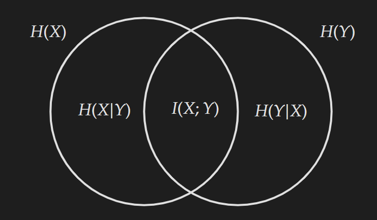
This diagram is used as a reference to explain mutual information. From the diagram, we can see mutual information $I(X; Y)$ is the overlapping region between $H(X)$ and $H(Y)$. This corresponds with the name mutual information as $H(X)$ is the expected self-information quantity in the random variable $X$ and $H(Y)$ is the expected self-information quantity in the random variable $Y$. Hence, the common section will be the “mutual information” which is shared by both random variables. Just by using common sense, without any prior knowledge, we can write down the following equations with the help of the Venn diagram:

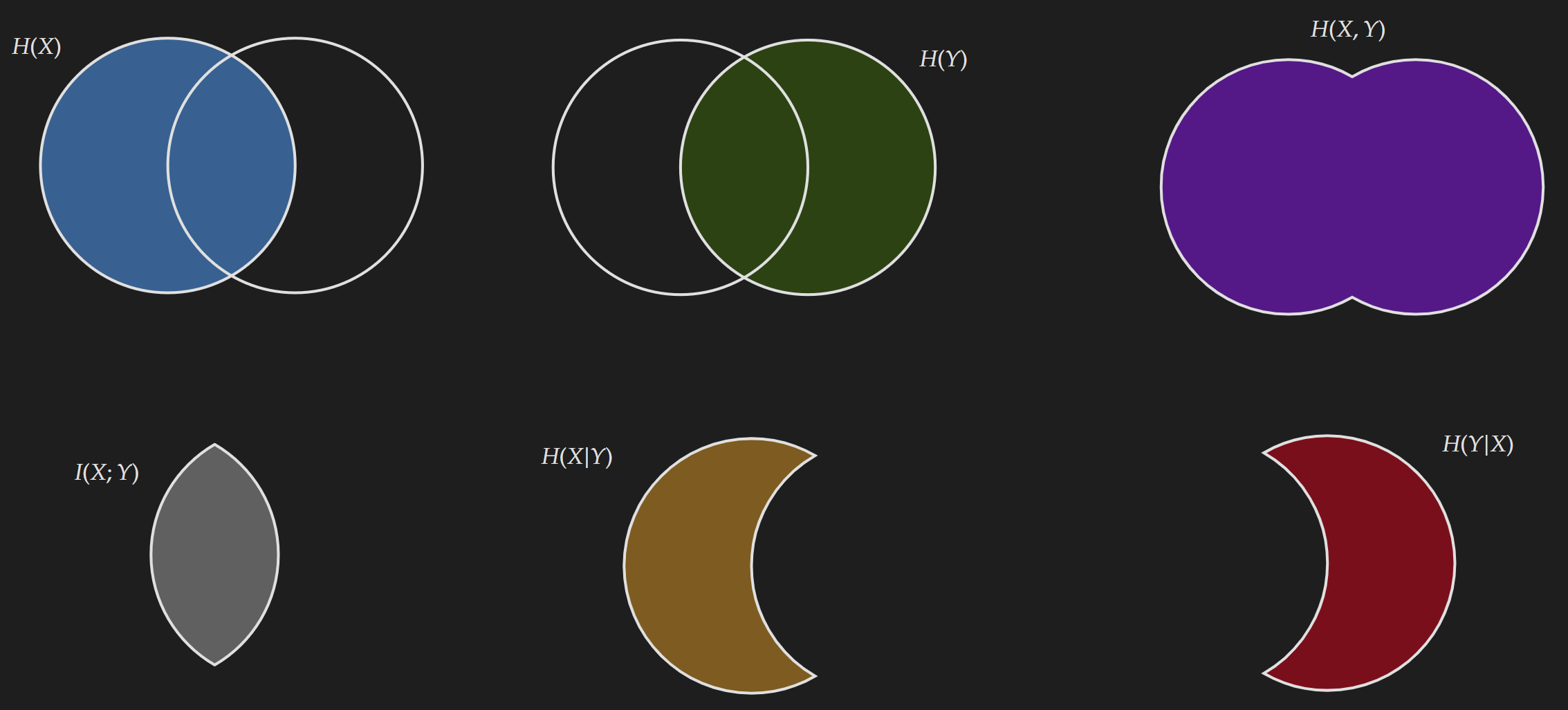
\[\begin{align*} I(X;Y)&= H(X)-H(X|Y)\\ &= H(Y)-H(Y|X) \\ &= H(X)+H(Y)-H(X,Y) \\ &=H(X, Y)-H(X \mid Y)-H(Y \mid X) \end{align*}\]

If you closely think about the above equations, all of them are essentially calculating the overlapped section. The following diagram highlighting different sections will make it more apparent.

The Formula

The formula for mutual information with respect to joint distribution and marginal distribution is shown below:

\[\boxed{\mathrm{I}(X ; Y)=\sum_{y \in \mathcal{Y}} \sum_{x \in \mathcal{X}} p{(x, y)} \log \left(\frac{p(x, y)}{p(x) p(y)}\right)}\]

This can be derived from the definitions of joint entropy, marginal entropy and conditional entropy. I am gonna provide a specific derivation, but know that this can be derived in many ways.

\[\begin{align*} I(X;Y) &= H(X)+H(Y)-H(X,Y)\\ & = \underbrace{-\sum_{x,y}p(x,y) \log p(x)}_{H(X)}\underbrace{-\sum_{x,y}p(x,y) \log p(y)}_{H(Y)}+\underbrace{\sum_{x,y}p(x,y) \log p(x,y)}_{-H(X,Y)} \\ &= \sum_{x,y}p(x,y) [\log p(x,y)-(\log p(x)+\log p(y))] \\ &= \sum_{x,y}p(x,y)\log \left(\frac{p(x, y)}{p(x) p(y)}\right) \\ \end{align*}\]

A significant observation that becomes apparent upon closer examination of the equation is what happens when the random variables $X$ and $Y$ are independent. When they are independent we know that $p(x,y)=p(x)p(y)$. Therefore, we get

\[I(X;Y)= \sum_{y \in \mathcal{Y}} \sum_{x \in \mathcal{X}} p{(x, y)} \log \left(1\right)=0\]

This means for independent random variables there is no mutual information; which is kind of obvious from the definition of mutual information.

$I(X,Y) \geq 0$ ; with equality iff $X$ and $Y$ are independent.

Normalized Mutual Information

Due to scale sensitivity and other issues with mutual information, it is preferable to work with a normalized version. However, in literature, there are many different ways NMI is calculated. These variations are based on the normalizing factor in the denominator. I will describe $4$ such versions which are available in Sckit-Learn.

\[NMI_{arithmetic}=\frac{ I(X; Y)}{\frac{H(X)+H(Y)}{2}}= \frac{ 2I(X; Y)}{H(X)+H(Y)}\]

Here the normalizing constant is the arithmetic mean of $H(X)$ and $H(Y)$ i.e. $\frac{H(X)+H(Y)}{2}$.

\[NMI_{geometric}=\frac{ I(X; Y)}{\sqrt{H(X)H(Y)}}\]

Here the normalizing constant is the geometric mean of $H(X)$ and $H(Y)$ i.e. $\sqrt{H(X)H(Y)}$.

\[NMI_{max} = \frac{ I(X; Y)}{max\{H(X),H(Y)\}}\]

Here the normalizing constant is the maximum of $H(X)$ and $H(Y)$.

\[NMI_{min} = \frac{ I(X; Y)}{min\{H(X),H(Y)\}}\]

Here the normalizing constant is the the minimum of $H(X)$ and $H(Y)$.